Oh, that place. It’s so crowded nobody goes there anymore.

Yogi Berra

If 2020 has given the world a phrase then that phrase is social distancing. However, it put me in mind of a classic analysis in economics/ complexity theory, the El Farol Bar problem.

I have long enjoyed running in Hyde Park. With social distancing I am aware that I need to time and route my runs to avoid crowds. The park is, legitimately, popular and a lot of people live within reasonable walking distance. Private gardens are at a premium in this part of West London. The pleasing thing is that people in general seem to have spread out their visits and the park tends not to get too busy, weather depending. It is almost as though the populace had some means of co-ordinating their visits. That said, I can assure you that I don’t phone up the several hundred thousand people who must live in the park’s catchment area.

The same applies to supermarket visits. Things seem to have stabilised. This put me in mind of W B Arthur’s 1994 speculative analysis of attendances at his local El Farol bar.¹ The bar was popular but generally seemed to be attended by a comfortable number of people, neither unpleasantly over crowded nor un-atmospherically quiet. This seems odd. Individual attendees had no obvious way of communicating or coordinating. If people, in general, believed that it would be over crowded then, pace Yogi Berra, nobody would go, thwarting their own expectations. But if there was a general belief it would be empty then everybody would go, again guaranteeing that their own individual forecasts were refuted.

Arthur asked himself how, given this analysis, people seemed to be so good at turning up in the right numbers. Individuals must have some way of predicting the attendance even though that barely seemed possible with the great number of independently acting people.

The model that Artur came up with was to endow every individual with an ecology of prediction formulas or rules, each taking the experience base and following a simple rule, using it to make a prediction of attendance the following week. Some of Arthur’s examples were, along with some others:

• Predict the same as last week’s attendance.
• Predict the average of the last 4 weeks’ attendances.
• Predict the same as the attendance 2 weeks ago.
• Add 5 to last week’s attendance.
• …

Now, every time an individual gets another week’s data he assesses the accuracy of the respective rules. He then adopts the currently most accurate rule to predict next week’s attendance.

Arthur ran a computer simulation. He set the optimal attendance at El Farol as 60. An individual predicting over 60 attendees would stay away. An individual predicting fewer would attend. He found that the time sequence of weekly attendances soon stabilised around 60.

There are a few points to pull out of that about human learning in general. What Arthur showed is that individuals, and communities thereof, have the ability to learn in an ill-defined environment in an unstructured way. Arthur was not suggesting that individuals co-ordinate by self-consciously articulating their theories and systematically updating on new data. He was suggesting the sort of unconscious and implicit decision mechanism that may inhabit the windmills of our respective minds. Mathematician and philosopher Alfred North Whitehead believed that much of society’s “knowledge” was tied up in such culturally embedded and unarticulated algorithms.²

It is a profoundly erroneous truism, repeated by all copy-books and by eminent people when they are making speeches, that we should cultivate the habit of thinking of what we are doing. The precise opposite is the case. Civilization advances by extending the number of important operations which we can perform without thinking about them. Operations of thought are like cavalry charges in a battle — they are strictly limited in number, they require fresh horses, and must only be made at decisive moments.

The regularity trap

Psychologists Gary Klein and Daniel Kahneman investigated how firefighters were able to perform so successfully in assessing a fire scene and making rapid, safety critical decisions. Lives of the public and of other firefighters were at stake. Together, Klein and Kahneman set out to describe how the brain could build up reliable memories that would be activated in the future, even in the agony of the moment. They came to the conclusion that there are two fundamental conditions for a human to acquire a predictive skill.³

• An environment that is sufficiently regular to be predictable.
• An opportunity to learn these regularities through prolonged practice

Arthur’s Fig.1, after the initial transient, looks impressively regular, stable and predictable. Some “invisible hand” has moved over the potential attendees and coordinated their actions. So it seems.

Though there is some fluctuation it is of a regular sort, what statisticians call exchangeable variation.

The power of a regular and predictable process is that it does enable us to keep Whitehead’s cavalry in reserve for what Kahneman called System 2 thinking, the reflective analytical dissection of a problem. It is the regularity that allows System 1 thinking where we can rely on heuristics, habits and inherited prejudices, the experience base.

The fascinating thing about the El Farol problem is that the regularity arises, not from anything consistent, but from data-adaptive selection from the ecology of rules. It is not obvious in advance that such can give rise to any, even apparent, stability. But there is a stability, and an individual can rely upon it to some extent. Certainly as far as a decision to spend a sociable evening is concerned. However, therein lies its trap.

Tastes in venue, rival attractions, new illnesses flooding the human race (pace Gottfried Leibniz), economic crises, … . Sundry matters can upset the regular and predictable system of attendance. And they will not be signalled in advance in the experience base.

Predicting on the basis of a robustly measured, regular and stable experience base will always be a hostage to emerging events. Agility in the face of emerging data-signals is essential. But understanding the vulnerabilities of current data patterns is important too. In risk analysis, understanding which historically stable processes are sensitive to foreseeable crises is essential.

Folk sociology

Folk physics is the name given to the patterns of behaviour that we all exhibit that enable us to catch projectiles, score “double tops” on the dart board, and which enabled Michel Platini to defy the wall with his free kicks. It is not the academic physics of Sir Isaac Newton which we learn in courses on theoretical mechanics and which enables the engineering of our most ambitious monumental structures. However, it works for us in everyday life, lifting boxes and pushing buggies.⁴

Apes, despite their apparently impressive ability to use tools, it turns out, have no internal dynamic models or physical theories at all. They are unable to predict in novel situations. They have no System 2 thinking. They rely on simple granular rules and heuristics, learned by observation and embedded by successful repetition. It seems more than likely that, in many circumstances, as advanced by Whitehead, that is true of humans too.⁵ Much of our superficially sophisticated behaviour is more habit than calculation, though habit in which is embedded genuine knowledge about our environment and successful strategies of value creation.⁶ Kahneman’s System 1 thinking.

The lesson of that is to respect what works. But where the experience base looks like the result of an pragmatic adjustment to external circumstances, indulge in trenchant criticism of historical data. And remain agile.

Next time I go out for a run, I’m going to check the weather.

References

1. Arthur, W B (1994) “Inductive reasoning and bounded rationality, The American Economic Review, 84 (2), Papers and Proceedings of the Hundred and Sixth Annual Meeting of the American Economic Association, 406-411
2. Whitehead, A N (1911) An Introduction to Mathematics, Ch.5
3. Kahneman, D (2011) Thinking, Fast and Slow, Allen Lane, p240
4. McCloskey (1983) “Intuitive physics”, Scientific American 248(4), 122-30
5. Povinelli, D J (2000) Folk Physics for Apes: The Chimpanzee’s Theory of How the World Works, Oxford
6. Hayek, F A (1945) “The use of knowledge in society”, The American Economic Review, 35(4), 519-530

In the words of the late, great Kenny Rogers, “There’ll be time enough for countin’/ When the dealin’s done”, but sometime, at the end of the Covid-19 crisis, somebody will ask How many died? and, more speculatively, how many deaths were avoidable.

There always seems an odd and uncomfortable premise at the base of that question, that somehow there is a natural or neutral, unmarked, control, null, default or proper, legitimate number who “should have” died, absent the virus. Yet that idea is challenged by our certain collective knowledge that, in living memory, there has been a persistent rise in life expectancy and longevity. Longevity has not stood still.

And I want to focus on that as it relates to a problem that has been bothering me for a while. It was brought into focus a few weeks ago by a headline in the Daily Mail, the UK’s house journal for health scares and faux consumer outrage.¹

Life expectancy in England has ground to a halt for the first time in a century, according to a landmark report.

For context, I should say that this appeared 8 days after the UK government’s first Covid-19 press conference. Obviously, somebody had an idea about how much life expectancy should be increasing. There was some felt entitlement to an historic pattern of improvement that had been, they said, interrupted. It seems that the newspaper headline was based on a report by Sir Michael Marmot, Professor of Epidemiology and Public Health at University College London.² This was Marmot’s headline chart.

Well, not quite the Daily Mail‘s “halt” but I think that there is no arguing with the chart. Despite there obviously having been some reprographic problem that has resulted in everything coming out in various shades of green and some gratuitous straight lines, it is clear that there was a break point around 2011. Following that, life expectancy has grown at a slower rate than before.

The chart did make me wonder though. The straight lines are almost too good to be true, like something from a freshman statistics service course. What happened in 2011? And what happened before 1980? Further, how is life expectancy for a baby born in 2018 being measured? I decided to go to the Office of National Statistics (UK) (“the ONS”) website and managed to find data back to 1841.

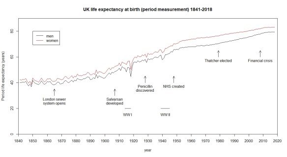
I have added some context but other narratives are available. Here is a different one.³

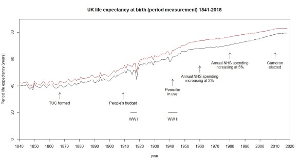
As Philip Tetlock⁴ and Daniel Kahneman⁵ have both pointed out, it is easy to find a narrative that fits both the data and our sympathies, and to use it as a basis for drawing conclusions about cause and effect. On the other hand, building a narrative is one of the most important components in understanding data. The way that data evolves over time and its linkage into an ecology of surrounding events is the very thing that drives our understanding of the cause system. Data has no meaning apart from its context. Knowledge of the cause system is critical to forecasting. But please use with care and continual trenchant criticism.

The first thing to notice from the chart is that there has been a relentless improvement in life expectancy over almost two centuries. However, it has not been uniform. There have been periods of relatively slow and relatively rapid growth. I could break the rate of improvement down into chunks as follows.

Here I have rather crudely fitted a straight line to the period measurement (I am going to come back to what this means) for men over the various epochs to a get a feel for the pace of growth. It is a very rough and ready approach. However, it does reveal that the real periods of improvement of life expectancy were from 1908 to 1948, notoriously the period of two World Wards and an unmitigated worldwide depression.

Other narratives are available.

It does certainly look as though improvement has slowed since the financial crisis of 2008. However, it has only gone back to the typical rate between 1948 and 1979, a golden age for some people I think, and nowhere near the triumphal march of the first half of the twentieth century. We may as well ask why the years 1980 to 2008 failed to match the heroic era.

There are some real difficulties in trying to come to any conclusions about cause and effect from this data.

Understanding the ONS numbers

In statistics, life expectancy is fully characterised by the survivor function. Once we know that, we can calculate everything we need, in particular life expectancy (mean life). Any decent textbook on survival analysis tells you how to do this.⁶ The survivor function tells us the probability that an individual will survive beyond time t and die at some later unspecified date. Survivor functions look like this, in general.

It goes from t=0 until the chances of survival have vanished, steadily decreasing with moral certainty. In fact, you can extract life expectancy (mean life) from this by measuring the area under the curve, perhaps with a planimeter.

However, what we are talking about is a survivor function that changes over time. Not in the sense that a survivor function falls away as an individual ages. A man born in 1841 will have a particular survivor function. A man born in 2018 will have a better one. We have a sequence of generally improving survivor functions over the years.

Now you will see the difficulty in estimating the survivor function for a man born in 1980. Most of them are still alive and we have nil data on that cohort’s specific fatalities after 40 years of age. Now, there are statistical techniques for handling that but none that I am going to urge upon you. Techniques not without their important limitations but useful in the right context. The difficulty in establishing a survivor function for a newborn in 2020 is all the more problematic. We can look at the age of everyone who dies in a particular year, but that sample will be a mixture of men born in each and every year over the preceding century or so. The individual years’ survivor functions will be “smeared” out by the instantaneous age distribution of the UK, what in mathematical terms is called convolution. That helps us understand why the trends seem, in general, well behaved. What we are looking at is the aggregate of effects over the preceding decades. There will, importantly in the current context, be some “instantaneous” effects from epidemics and wars but those are isolated events within the general smooth trend of improvement.

There is no perfect solution to these problems. The ONS takes two approaches both of which it publishes.⁷ The first is just to regard the current distribution of ages at death as though it represented the survivor function for a person born this year. This, of course, is a pessimistic outlook for a newborn’s prospects. This year’s data is a mixture of the survivor functions for births over the last century or so, along with instantaneous effects. For much of those earlier decades, life expectancy was signally worse than it is now. However, the figure does give a conservative view and it does enable a year-on-year comparison of how we are doing. It captures instantaneous effects well. The ONS actually take the recorded deaths over the last three consecutive years. This is what they refer to as the period measurement and it is what I have used in this post.

The other method is slightly more speculative in that it attempts to reconstruct a “true” survivor function but is forced into making that through assuming an overall secular improvement in longevity. This is called the cohort measurement. The ONS use historical life data then assume that the annual rate of increase in life expectancy will be 1.2% from 2043 onwards. Rates between 2018 and 2043 are interpolated. The cohort measurement yields a substantially higher life expectancy than the period measurement, 87.8 years as against 79.5 years for 2018 male births.

Endogenous and exogenous improvement

Well, I really hesitated before I used those two economists’ terms but they are probably the most scholarly. I shall try to put it more cogently.

There is improvement contrived by endeavour. We identify some desired problem, conceive a plausible solution, implement, then measure the results against the pre-solution experience base. There are many established processes for this, DMAIC is a good one, but there is no reason to be dogmatic as to approach.

However, some improvement occurs because there is an environment of appropriate market conditions and financial incentives. It is the environment that is important in turning random, and possibly unmotivated, good ideas into improvement. As German sociologist Max Weber famously observed, “Ideas occur to us when they please, not when it pleases us.”⁸

For example, in 1858, engineer Joseph Bazalgette proposed an enclosed, underground sewer system for much of London. A causative association between fecal-contaminated water and cholera had been current since the work of John Snow in 1854. That’s another story. Bazalgette’s engineering was instrumental in relieving the city from cholera. That is an improvement procured by endeavour, endogenous if you like.

In 1928, Sir Alexander Fleming noticed how mould, accidentally contaminating his biological samples, seemed to inhibit bacterial growth. Fleming pursued this random observation and ended up isolating penicillin. However, it took a broader environment of value, demand and capital to launch penicillin as a pharmaceutical product, some time in the 1940s. There were critical stages of clinical trials and industrial engineering demanding significant capital investment and constancy of purpose. Howard Florey, Baron Florey, was instrumental and, in many ways, his contribution is greater than Fleming’s. However, penicillin would not have reached the public had the market conditions not been there. The aggregate of incremental improvements arising from accidents of discovery, nurtured by favourable external  economic and political forces, are the exogenous improvements. All the partisans will claim success for their party.

Of course, it is, to some extent, a fuzzy characterisation. Penicillin required Florey’s (endogenous) endeavour. All endeavour takes place within some broader (exogenous) culture of improvement. Paul Ehrlich hypothesised that screening an array of compounds could identify drugs with anti-bacterial properties. Salvarsan’s effectiveness against syphilis was discovered as part of such a programme and then developed and marketed as a product by Hoechst in 1910. An interaction of endogenous and exogenous forces.

It is, for business people who know their analytics, relatively straightforward to identify improvements from endogenous endeavour. But where they dynamics are exogenous, economists can debate and politicians celebrate or dispute. Improvements can variously be claimed on behalf of labour law, state aid, nationalisation, privatisation or market deregulation. Then, is the whole question of cause and effect slightly less obvious than we think? Moderns carol the innovation of penicillin. We shudder noting that, in 1924, a US President’s son died simply because of an infection originating in an ill-fitting tennis shoe.⁹ However, looking at the charts of life expectancy, there is no signal from the introduction of penicillin, I think. What caused that improvement in the first half of the twentieth century?

Cause and effect

It was philosopher-scientist-lawyer Francis Bacon who famously observed:

It were infinite for the law to judge the causes of causes and the impression one on another.

We lawyers are constantly involved in disputes over cause and effect. We start off by accepting that nearly everything that happens is as a result of many causes. Everyday causation is inevitably a multifactorial matter. That is why the cause and effect diagram is essential to any analysis, in law, commerce or engineering. However, lawyers are usually concerned with proving that a particular factor caused an outcome. Other factors there may be and that may well be a matter of contribution from other parties but liability turns on establishing that a particular action was part of the causative nexus.

The common law has some rather blunt ways of dealing with the matter. Pre-eminent is the “but for” test. We say that A caused B if B would not have happened but for A. There may well have been other causes of B, even ones that were more important, but it is A that is under examination. That though leaves us with, at least, a couple of problems. Lord Hoffman pointed out the first problem in South Australia Asset Management Corporation Respondents v York Montague Ltd.¹⁰

A mountaineer about to take a difficult climb is concerned about the fitness of his knee. He goes to the doctor who makes a superficial examination and pronounces the knee fit. The climber goes on the expedition, which he would not have undertaken if the doctor told him the true state of his knee. He suffers an injury which is an entirely foreseeable consequence of mountaineering but has nothing to do with his knee.

The law deals with this by various devices: operative cause, remoteness and foreseeability,  reasonable foreseeability, reasonable contemplation of the parties, breaks in the chain of causation, boundaries on the duty of care … . The law has to draw a line and avoid “opening the floodgates” of liability.^{11, 12} How the line can be drawn objectively in social science is a different matter.

The second issue was illustrated in a fine analysis by Prof. David Spiegelhalter as to headlines of 40,000 annual UK deaths because of air pollution.¹³ Daily Mail again! That number had been based on historical longitudinal observational studies showing greater force of mortality among those with greater exposure to particular pollutants. I presume, though Spiegelhalter does not go into this in terms, that there is some plausible physio-chemical cause system that can describe the mechanism of action of inhaled chemicals on metabolism and the risk of early death.

Thus we can expose a population to a risk with a moral certainty that more will die than absent the risk. That does not, of itself, enable us to attribute any particular death to the exposure. There may, in any event, be substantial uncertainty about the exact level of risk.

The law is emphatic. Mere exposure to a risk is insufficient to establish causation and liability.¹⁴ There are a few exceptions. I will not go into them here. The law is willing to find causation in situations that fall short of but for where it finds that the was a material contribution to a loss.¹⁵ However, a claimant must, in general, show a physical route to the individual loss or injury.¹⁶

A question of attribution

Thus, even for those with Covid-19 on their death certificate, the cause will typically be multi-factorial. Some would have died in the instant year in any event. And some others will die because medical resources have been diverted from the quotidian treatment of the systemic perils of life. The local disruption, isolation, avoidance and confinement may well turn out to result in further deaths. Domestic violence is a salient repercussion of this pandemic.

But there is something beyond that. One of Marmot’s principle conclusions was that the recent pause in improvement of life expectancy was the result of poverty. In general, the richer a community becomes, the longer it lives. Poverty is a real factor in early death. On 14 April 2020, the UK Office of Budget Responsibility opined that the UK economy could shrink by 35% by June.¹⁷ There was likely to be a long lasting impact on public finances. Such a contraction would dwarf even the financial crisis of 2008. If the 2008 crisis diminished longevity, what will a Covid-19 depression do? How will deaths then be attributed to the virus?

The audit of Covid-19 deaths is destined to be controversial, ideological, partisan and likely bitter. The data, once that has been argued over, will bear many narratives. There is no “right” answer to this. An honest analysis will embrace multiple accounts and diverse perspectives. We live in hope.

I think it was Jack Welch who said that anybody could manage the short term and anybody could manage the long term. What he needed were people who could manage the short term and the long term at the same time.

References

1. “Life expectancy grinds to a halt in England for the first time in 100 YEARS”, Daily Mail , 25/2/20, retrieved 13/4/20
2. Marmot, M et al. (2020) Health Equity in England: The Marmot Review 10 Years On, Institute of Health Equity
3. NHS expenditure data from, “How funding for the NHS in the UK has changed over a rolling ten year period”, The Health Foundation, 31/10/15, retrieved 14/4/20
4. Tetlock, P & Gardner, D (2015) Superforecasting: The Art and Science of Prediction, Random House
5. Kahneman, D (2011) Thinking, fast and slow, Allen Lane
6. Mann, N R et al. (1974) Methods for Statistical Analysis of Reliability and Life Data, Wiley
7. “Period and cohort life expectancy explained”, ONS, December 2019, retrieved 13/4/20
8. Weber, M (1922) “Science as a vocation”, in Gessamelte Aufsätze zur Wissenschaftslehre, Tubingen, JCB Mohr 1922, 524-555
9. The medical context of Calvin Jr’s untimely death“, Coolidge Foundation, accessed 13/4/20
10. [1997] AC 191 at 213
11. Charlesworth & Percy on Negligence, 14th ed., 2-03
12. Lamb v Camden LBC [1981] QB 625, per Lord Denning at 636
13. “Does air pollution kill 40,000 people each year in the UK?”, D Siepgelhalter, Medium, 20/2/17, retrieved 13/4/20
14. Wilsher v Essex Area Health Authority [1988] AC 1075, HL
15. Bailey v Ministry of Defence [2008] EWCA Civ 883, [2009] 1 WLR 1052
16. Pickford v ICI [1998] 1 WLR 1189, HL
17. “Coronavirus: UK economy ‘could shrink by record 35%’ by June”, BBC News 14/4/20, retrieved 14/4/20

If anybody doubts that twitter has a valuable role in the world they should turn their attention to the twitter sensation that is @justsaysinmice.

The twitter feed exposes bad science journalism where extravagant claims are advanced with a penumbra of implication that something relevant to human life or happiness has been certified by peer reviewed science. It often turns out that, when the original research in interrogated, and in fairness at the very bottom of the journalistic puff piece, it just says, “in mice”. Cauliflower, cabbage, broccoli harbour prostate cancer inhibiting compound, was a recent subeditor’s attention grabbing headline. But the body of the article just says, “in mice”. Most days the author finds at least one item to tweet.

Population – Frame – Sample

The big point here is one of the really big points in understanding statistics.

We start generating data and doing statistics because there is something out there we are interested in. Some things or events. We call the things and events we are bothered about the population. The problem is that, in the real world, it is often difficult to get hold of all those things or events. In an opinion poll, we don’t know who will vote at the next election, or even who will still be alive. We don’t know all the people who follow a particular sports club. We can’t find everyone who’s ever tasted Marmite and expressed an opinion. Sometimes the events or things we are interested in don’t even exist yet and lie wholly in the future. That’s called prediction and forecasting.

In order to do the sort of statistical sampling that text books tell us about, we need to identify some relevant material that is available to us to measure or interrogate. For the opinion poll it would be everyone on the electoral register, perhaps. Or everyone who can be reached by dialing random numbers in the region of interest. Or everyone who signs up to an online database (seriously). Those won’t be the exact people who will be doing the voting at the next election. Some of them likely will be. But we have to make a judgment that they are, somehow, representative.

Similarly, if we want to survey sports club supporters we could use the club’s supporter database. Or the people who but tickets online. Or who tweet. Not perfect but, hey! And, perhaps, in some way representative.

The collection of things we are going to do the sampling on is called the sampling frame. We don’t need to look at the whole of the frame. We can sample. And statistical theory assures us about how much the sample can tell us about the frame, usually quite a lot if done properly. But as to the differences between population and frame, that is another question.

Enumerative and analytic statistics

These real world situations lie in contrast to the sort of simplified situations found in statistics text books. A inspector randomly samples 5 widgets from a batch of 100 and decides whether to accept or reject the batch (though why anyone would do this still defies rational explanation). Here the frame and population are identical. No need to worry.

W Edwards Deming was a statistician who, among his other achievements, developed the sampling techniques used in the 1940 US census. Deming thought deeply about sampling and continually emphasised the distinction between the sort of problems where population and frame were identical, what he called enumerative statistics, and the sundry real world situations where they were not, analytic statistics.¹

The key to Deming’s thinking is that, where we are doing analytic statistics, we are not trying to learn about the frame, that is not what interests us, we are trying to learn something useful about the population of concern. That means that we have to use the frame data to learn about the cause system that is common to frame and population. By cause system, Deming meant the aggregate of competing, interacting and evolving factors, inherent and environmental, that influence the outcomes both in frame and population. As Donald Rumsfeld put it, the known knowns, the known unknowns and the unknown unknowns.

The task of understanding how any particular frame and population depend on a common cause-system requires deep subject matter knowledge. As does knowing the scope for reading across conclusions.

Just says, “in mice”

Experimenting on people is not straightforward. That’s why we do experiments on mice.

But here the frame and population are wildly disjoint.
So why? Well apparently, their genetic, biological and behavior characteristics closely resemble those of humans, and many symptoms of human conditions can be replicated in mice.² That is, their cause systems have something in common. Not everything but things useful to researchers and subject matter experts.

Now, that means that experimental results in mice can’t just be read across as though we had done the experiment on humans. But they help subject matter experts learn more about those parts of the cause-system that are common. That might then lead to tentative theories about human welfare that can then be tested in the inevitably more ethically stringent regime of human trials.

So, not only is bad, often sensationalist, data journalism exposed, but we learn a little more about how science is done.

Just says, “in boys”

If the importance of this point needed emphasising then Caroline Criado Perez makes the case compellingly in her recent book Invisible Women.³

It turns out, that much medical research, much development of treatments and even assessment of motor vehicle safety have historically been performed on frames dominated by men, but with results then read across as though representative of men and women. Perez goes on to show how this has made women’s lives less safe and less healthy than they need have been.

It seems that it is not only journalists who are addicted to bad science.

Anyone doing statistics needs aggressively to scrutinise their sampling frame and how it matches the population of interest. Contrasts in respective cause systems need to be interrogated and distinguished with domain knowledge, background information and contextual data. Involvement in statistics carries responsibilities.

References

1. Deming, W E (1975) “On probability as a basis for action”, American Statistician, 29 146
2. Melina, R (2010) “Why Do Medical Researchers Use Mice?“, Live Science, retrieved 18:32 UCT 2/6/19
3. Perez, C C (2019) Invisible Women: Exposing Data Bias in a World Designed for Men, Chatto & Windus

References

1. Kennedy, J (2019) Populist politics and vaccine hesitancy in Western Europe: an analysis of national-level data, Journal of Public Health, ckz004, https://doi.org/10.1093/eurpub/ckz004
2. Semmelweis, I (1860) The Etiology, Concept, and Prophylaxis of Childbed Fever, trans. K Codell Carter [1983] University of Wisconsin Press: Madison, Wisconsin
3.  Kerr, W A & Hobbs, J E (2005). “9. Consumers, Cows and Carousels: Why the Dispute over Beef Hormones is Far More Important than its Commercial Value”, in Perdikis, N & Read, R, The WTO and the Regulation of International Trade. Edward Elgar Publishing, pp 191–214
4. Caduff, L (August 2002). “Growth Hormones and Beyond” (PDF). ETH Zentrum. Archived from the original (PDF) on 25 May 2005. Retrieved 11 December 2007.
5. Gandhi, R & Snedeker, S M (June 2000). “Consumer Concerns About Hormones in Food“. Program on Breast Cancer and Environmental Risk Factors. Cornell University. Archived from the original on 19 July 2011.
6. I J Good
7. Kahneman, D (2011) Thinking, Fast and Slow, London: Allen Lane, pp80-81
UK railway suicides – 2018 update
The latest UK rail safety statistics were published on 6 December 2018, again absent much of the press fanfare we had seen in the past. Regular readers of this blog will know that I have followed the suicide data series, and the press response, closely in 2017, 2016, 2015, 2014, 2013 and 2012. Again I have re-plotted the data myself on a Shewhart chart.
RailwaySuicides20181
Readers should note the following about the chart.
• Many thanks to Tom Leveson Gower at the Office of Rail and Road who confirmed that the figures are for the year up to the end of March.
• Some of the numbers for earlier years have been updated by the statistical authority.
• I have recalculated natural process limits (NPLs) as there are still no more than 20 annual observations, and because the historical data has been updated. The NPLs have therefore changed but, this year, not by much.
• Again, the pattern of signals, with respect to the NPLs, is similar to last year.
The current chart again shows the same two signals, an observation above the upper NPL in 2015 and a run of 8 below the centre line from 2002 to 2009. As I always remark, the Terry Weight rule says that a signal gives us license to interpret the ups and downs on the chart. So I shall have a go at doing that.
After two successive annual falls there has been an increase in the number of fatalities.
I haven’t yet seen any real contemporaneous comment on the numbers from the press this year. But what conclusions can we really draw?
In 2015 I was coming to the conclusion that the data increasingly looked like a gradual upward trend. The 2016 and 2017 data offered a challenge to that but my view was still that it was too soon to say that the trend had reversed. There was nothing in the data incompatible with a continuing trend. The decline has not continued but how much can we read into that? There is nothing inherently informative about a relative increase. Remember, the data would certainly have gone up or down. Then again, was there some sort of peak in 2015?
Signal or noise?
Has there been a change to the underlying cause system that drives the suicide numbers? Since the 2016 data, I have fitted a trend line through the data and asked which narrative best fitted what I observed, a continuing increasing trend or a trend that had plateaued or even reversed. You can review my analysis from 2016 here. And from 2017 here.
Here is the data and fitted trend updated with this year’s numbers, along with NPLs around the fitted line, the same as I did in 2016 and 2017.
RailwaySuicides20182
We always go back to the cause and effect diagram.
SuicideCne
As I always emphasise, the difficulty with the suicide data is that there is very little reproducible and verifiable knowledge as to its causes. There is a lot of useful thinking from common human experience and from more general theories in psychology. But the uncertainty is great. It is not possible to come up with a definitive cause and effect diagram on which all will agree, other from the point of view of identifying candidate factors. In statistical terminology, the problem lacks rigidity.
The earlier evidence of a trend, however, suggests that there might be some causes that are developing over time. It is not difficult to imagine that economic trends and the cumulative awareness of other fatalities might have an impact. We are talking about a number of things that might appear on the cause and effect diagram and some that do not, the “unknown unknowns”. When I identified “time” as a factor, I was taking sundry “lurking” factors and suspected causes from the cause and effect diagram that might have a secular impact. I aggregated them under the proxy factor “time” for want of a more refined analysis.
What I have tried to do is to split the data into two parts:
• A trend (linear simply for the sake of exploratory data analysis (EDA)); and
• The residual variation about the trend.
The question I want to ask is whether the residual variation is stable, just plain noise, or whether there is a signal there that might give me a clue that a linear trend does not hold.
There is no signal in the detrended data, no signal that the trend has reversed. The tough truth of the data is that it supports either narrative.
• The upward trend is continuing and is stable. There has been no reversal of trend yet.
• The raw data is not stable. True there is evidence of an upward trend in the past but there is now evidence that deaths are decreasing, notwithstanding the increase over the last year.
Of course, there is no particular reason, absent the data, to believe in an increasing trend and the initiative to mitigate the situation might well be expected to result in an improvement.
Sometimes, with data, we have to be honest and say that we do not have the conclusive answer. That is the case here. All that can be done is to continue the existing initiatives and look to the future. Nobody ever likes that as a conclusion but it is no good pretending things are unambiguous when that is not the case.
Next steps
Previously I noted proposals to repeat a strategy from Japan of bathing railway platforms with blue light. In the UK, I understand that such lights were installed at Gatwick in summer 2014. There is some recent commentary here from the BBC but I feel the absence of any real systematic follow up on this. I have certainly seen nothing from Gatwick. My wife and I returned through there mid-January this year and the lights are still in place.
A huge amount of sincere endeavour has gone into this issue but further efforts have to be against the background that there is still no conclusive evidence of improvement.
Suggestions for alternative analyses are always welcomed here.