Don Wheeler coined the term executive time series. I was just leaving court in Oxford the other day when I saw this announcement on a hoarding. I immediately thought to myself “#executivetimeseries”.
Wheeler introduced the phrase in his 2000 book Understanding Variation: The Key to Managing Chaos. He meant to criticise the habitual way that statistics are presented in business and government. A comparison is made between performance at two instants in time. Grave significance is attached as to whether performance is better or worse at the second instant. Well, it was always unlikely that it would be the same.
The executive time series has the following characteristics.
- It as applied to some statistic, metric, Key Performance Indicator (KPI) or other measure that will be perceived as important by its audience.
- Two time instants are chosen.
- The statistic is quoted at each of the two instants.
- If the latter is greater than the first then an increase is inferred. A decrease is inferred from the converse.
- Great significance is attached to the increase or decrease.
Why is this bad?
At its best it provides incomplete information devoid of context. At its worst it is subject to gross manipulation. The following problems arise.
- Though a signal is usually suggested there is inadequate information to infer this.
- There is seldom explanation of how the time points were chosen. It is open to manipulation.
- Data is presented absent its context.
- There is no basis for predicting the future.
The Oxford billboard is even worse than the usual example because it doesn’t even attempt to tell us over what period the carbon reduction is being claimed.
Signal and noise
Let’s first think about noise. As Daniel Kahneman put it “A random event does not … lend itself to explanation, but collections of random events do behave in a highly regular fashion.” Noise is a collection of random events. Some people also call it common cause variation.
Imagine a bucket of thousands of beads. Of the beads, 80% are white and 20%, red. You are given a paddle that will hold 50 beads. Use the paddle to stir the beads then draw out 50 with the paddle. Count the red beads. Repeat this, let us say once a week, until you have 20 counts. The data might look something like this.
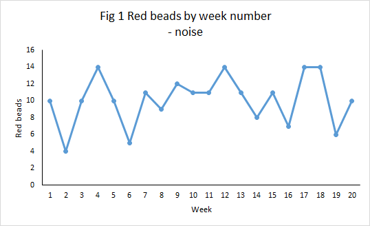
What we observe in Figure 1 is the irregular variation in the number of red beads. However, it is not totally unpredictable. In fact, it may be one of the most predictable things you have ever seen. Though we cannot forecast exactly how many red beads we will see in the coming week, it will most likely be in the rough range of 4 to 14 with rather more counts around 10 than at the extremities. The odd one below 4 or above 14 would not surprise you I think.
But nothing changed in the characteristics of the underlying process. It didn’t get better or worse. The percentage of reds in the bucket was constant. It is a stable system of trouble. And yet measured variation extended between 4 and 14 red beads. That is why an executive time series is so dangerous. It alleges change while the underlying cause-system is constant.
Figure 2 shows how an executive time series could be constructed in week 3.
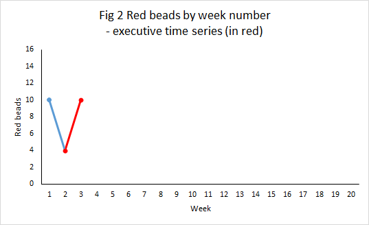
The number of beads has increase from 4 to 10, a 150% increase. Surely a “significant result”. And it will always be possible to find some managerial initiative between week 2 and 3 that can be invoked as the cause. “Between weeks 2 and 3 we changed the angle of inserting the paddle and it has increased the number of red beads by 150%.”
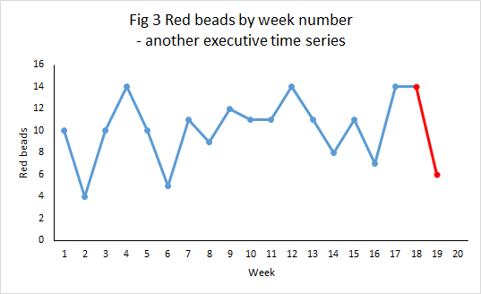
But Figure 2 is not the only executive time series that the data will support. In Figure 3 the manager can claim a 57% reduction from 14 to 6. More than the Oxford banner. Again, it will always be possible to find some factor or incident supposed to have caused the reduction. But nothing really changed.
The executive can be even more ambitious. “Between week 2 and 17 we achieved a 250% increase in red beads.” Now that cannot be dismissed as a mere statistical blip.

#executivetimeseries
Data has no meaning apart from its context.
Not everyone who cites an executive time series is seeking to deceive. But many are. So anybody who relies on an executive times series, devoid of context, invites suspicion that they are manipulating the message. This is Langian statistics. par excellence. The fallacy of What you see is all there is. It is essential to treat all such claims with the utmost caution. What properly communicates the present reality of some measure is a plot against time that exposes its variation, its stability (or otherwise) and sets it in the time context of surrounding events.
We should call out the perpetrators. #executivetimeseries
Techie note
The data here is generated from a sequence of 20 Bernoulli experiments with probability of “red” equal to 0.2 and 50 independent trials in each experiment.
 A supposed corollary to the