Regression done right: Part 2: Is it worth the trouble?

In Part 1 I looked at linear regression from the point of view of machine learning and asked the question whether the data was from “An environment that is sufficiently regular to be predictable.”1 The next big question is whether it was worth it in the first place.

Variation explained

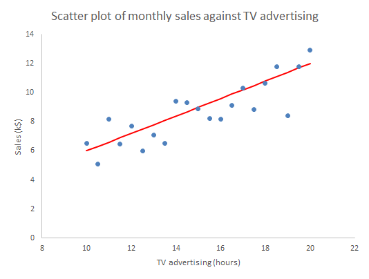
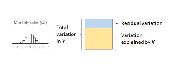
We previously looked at regression in terms of explaining variation. The original Big Y was beset with variation and uncertainty. We believed that some of that variation could be “explained” by a Big X. The linear regression split the variation in Y into variation that was explained by X and residual variation whose causes are as yet obscure.

I slipped in the word “explained”. Here it really means that we can draw a straight line relationship between X and Y. Of course, it is trite analytics that “association is not causation”. As long ago as 1710, Bishop George Berkeley observed that:2

The Connexion of Ideas does not imply the Relation of Cause and Effect, but only a Mark or Sign of the Thing signified.

Causation turns out to be a rather slippery concept, as all lawyers know, so I am going to leave it alone for the moment. There is a rather good discussion by Stephen Stigler in his recent book The Seven Pillars of Statistical Wisdom.3

That said, in real world practical terms there is not much point bothering with this if the variation explained by the X is small compared to the original variation in the Y with the majority of the variation still unexplained in the residuals.

Measuring variation

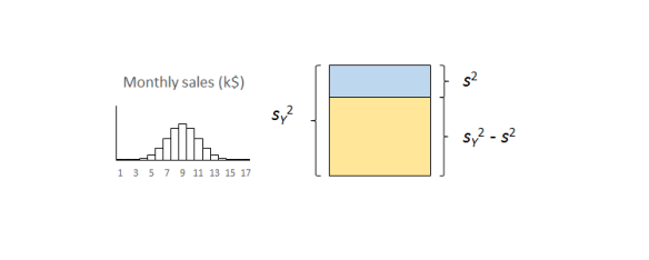
A useful measure of the variation in a quantity is its variance, familiar from the statistics service course. Variance is a good straightforward measure of the financial damage that variation does to a business.4 It also has the very nice property that we can add variances from sundry sources that aggregate together. Financial damage adds up. The very useful job that linear regression does is to split the variance of Y, the damage to the business that we captured with the histogram, into two components:

  • The contribution from X; and
  • The contribution of the residuals.

RegressionBlock1
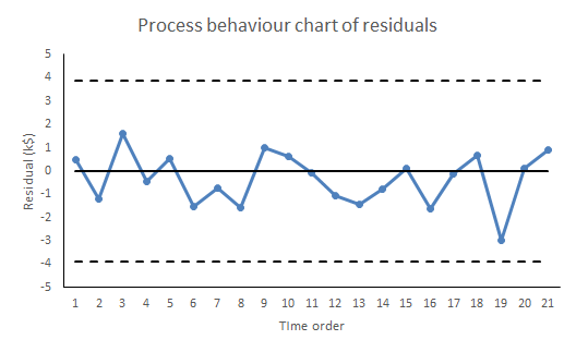
The important thing to remember is that the residual variation is not some sort of technical statistical artifact. It is the aggregate of real world effects that remain unexamined and which will continue to cause loss and damage.

RegressionIshikawa2

Techie bit

Variance is the square of standard deviation. Your linear regression software will output the residual standard deviation, s, sometimes unhelpfully referred to as the residual standard error. The calculations are routine.5 Square s to get the residual variance, s2. The smaller is s2, the better. A small s2 means that not much variation remains unexplained. Small s2 means a very good understanding of the cause system. Large s2 means that much variation remains unexplained and our understanding is weak.
RegressionBlock2

The coefficient of determination

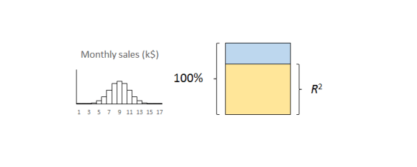
So how do we decide whether s2 is “small”? Dividing the variation explained by X by the total variance of Y, sY2,  yields the coefficient of determination, written as R2.6 That is a bit of a mouthful so we usually just call it “R-squared”. R2 sets the variance in Y to 100% and expresses the explained variation as a percentage. Put another way, it is the percentage of variation in Y explained by X.

RegressionBlock3The important thing to remember is that the residual variation is not a statistical artifact of the analysis. It is part of the real world business system, the cause-system of the Ys.7 It is the part on which you still have little quantitative grasp and which continues to hurt you. Returning to the cause and effect diagram, we picked one factor X to investigate and took its influence out of the data. The residual variation is the variation arising from the aggregate of all the other causes.

As we shall see in more detail in Part 3, the residual variation imposes a fundamental bound on the precision of predictions from the model. It turns out that s is the limiting standard error of future predictions

Whether your regression was a worthwhile one or not so you will want to probe the residual variation further. A technique like DMAIC works well. Other improvement processes are available.

So how big should R2 be? Well that is a question for your business leaders not a statistician. How much does the business gain financially from being able to explain just so much variation in the outcome? Anybody with an MBA should be able to answer this so you should have somebody in your organisation who can help.

The correlation coefficient

Some people like to take the square root of R2 to obtain what they call a correlation coefficient. I have never been clear as to what this was trying to achieve. It always ends up telling me less than the scatter plot. So why bother? R2 tells me something important that I understand and need to know. Leave it alone.

What about statistical significance?

I fear that “significance” is, pace George Miller, “a word worn smooth by many tongues”. It is a word that I try to avoid. Yet it seems a natural practice for some people to calculate a p-value and ask whether the regression is significant.

I have criticised p-values elsewhere. I might calculate them sometimes but only because I know what I am doing. The terrible fact is that if you collect sufficient data then your regression will eventually be significant. Statistical significance only tells me that you collected a lot of data. That’s why so many studies published in the press are misleading. Collect enough data and you will get a “significant” result. It doesn’t mean it matters in the real world.

R2 is the real world measure of sensible trouble (relatively) impervious to statistical manipulation. I can make p as small as I like just by collecting more and more data. In fact there is an equation that, for any given R2, links p and the number of observations, n, for linear regression.8

FvR2 equation

Here, Fμ, ν(x) is the F-distribution with μ and ν degrees of freedom. A little playing about with that equation in Excel will reveal that you can make p as small as you like without R2 changing at all. Simply by making n larger. Collecting data until p is small is mere p-hacking. All p-values should be avoided by the novice. R2 is the real world measure (relatively) impervious to statistical manipulation. That is what I am interested in. And what your boss should be interested in.

Next time

Once we are confident that our regression model is stable and predictable, and that the regression is worth having, we can move on to the next stage.

Next time I shall look at prediction intervals and how to assess uncertainty in forecasts.

References

  1. Kahneman, D (2011) Thinking, Fast and Slow, Allen Lane, p240
  2. Berkeley, G (1710) A Treatise Concerning the Principles of Human Knowledge, Part 1, Dublin
  3. Stigler, S M (2016) The Seven Pillars of Statistical Wisdom, Harvard University Press, pp141-148
  4. Taguchi, G (1987) The System of Experimental Design: Engineering Methods to Optimize Quality and Minimize Costs, Quality Resources
  5. Draper, N R & Smith, H (1998) Applied Regression Analysis, 3rd ed., Wiley, p30
  6. Draper & Smith (1998) p33
  7. For an appealing discussion of cause-systems from a broader cultural standpoint see: Bostridge, I (2015) Schubert’s Winter Journey: Anatomy of an Obsession, Faber, pp358-365
  8. Draper & Smith (1998) p243
Advertisement

Regression done right: Part 1: Can I predict the future?

I recently saw an article in the Harvard Business Review called “Refresher on Regression Analysis”. I thought it was horrible so I wanted to set the record straight.

Linear regression from the viewpoint of machine learning

Linear regression is important, not only because it is a useful tool in itself, but because it is (almost) the simplest statistical model. The issues that arise in a relatively straightforward form are issues that beset the whole of statistical modelling and predictive analytics. Anyone who understands linear regression properly is able to ask probing questions about more complicated models. The complex internal algorithms of Kalman filters, ARIMA processes and artificial neural networks are accessible only to the specialist mathematician. However, each has several general features in common with simple linear regression. A thorough understanding of linear regression enables a due diligence of the claims made by the machine learning advocate. Linear regression is the paradigmatic exemplar of machine learning.

There are two principal questions that I want to talk about that are the big takeaways of linear regression. They are always the first two questions to ask in looking at any statistical modelling or machine learning scenario.

  1. What predictions can I make (if any)?
  2. Is it worth the trouble?

I am going to start looking at (1) in this blog and complete it in a future Part 2. I will then look at (2) in a further Part 3.

Variation, variation, variation

Variation is a major problem for business, the tendency of key measures to fluctuate irregularly. Variation leads to uncertainty. Will the next report be high or low? Or in the middle? Because of the uncertainty we have to allow safety margins or swallow some non-conformancies. We have good days and bad days, good products and not so good. We have to carry costly working capital because of variation in cash flow. And so on.

We learned in our high school statistics class to characterise variation in a key process measure, call it the Big Y, by an histogram of observations. Perhaps we are bothered by the fluctuating level of monthly sales.

RegressionHistogram

The variation arises from a whole ecology of competing and interacting effects and factors that we call the cause-system of the outcome. In general, it is very difficult to single out individual factors as having been the cause of a particular observation, so entangled are they. It is still useful to capture them for reference on a cause and effect diagram.

RegressionIshikawa

One of the strengths of the cause and effect diagram is that it may prompt the thought that one of the factors is particularly important, call it Big X, perhaps it is “hours of TV advertising” (my age is showing). Motivated by that we can generate a sample of corresponding measurements data of both the Y and X and plot them on a scatter plot.

RegressionScatter1

Well what else is there to say? The scatter plot shows us all the information in the sample. Scatter plots are an important part of what statistician John Tukey called Exploratory Data Analysis (EDA). We have some hunches and ideas, or perhaps hardly any idea at all, and we attack the problem by plotting the data in any way we can think of. So much easier now than when W Edwards Deming wrote:1

[Statistical practice] means tedious work, such as studying the data in various forms, making tables and charts and re-making them, trying to use and preserve the evidence in the results and to be clear enough to the reader: to endure disappointment and discouragement.

Or as Chicago economist Ronald Coase put it.

If you torture the data enough, nature will always confess.

The scatter plot is a fearsome instrument of data torture. It tells me everything. It might even tempt me to think that I have a basis on which to make predictions.

Prediction

In machine learning terms, we can think of the sample used for the scatter plot as a training set of data. It can be used to set up, “train”, a numerical model that we will then fix and use to predict future outcomes. The scatter plot strongly suggests that if we know a future X alone we can have a go at predicting the corresponding future Y. To see that more clearly we can draw a straight line by hand on the scatter plot, just as we did in high school before anybody suggested anything more sophisticated.

RegressionScatter2

Given any particular X we can read off the corresponding Y.

RegressionScatter3

The immediate insight that comes from drawing in the line is that not all the observations lie on the line. There is variation about the line so that there is actually a range of values of Y that seem plausible and consistent for any specified X. More on that in Parts 2 and 3.

In understanding machine learning it makes sense to start by thinking about human learning. Psychologists Gary Klein and Daniel Kahneman investigated how firefighters were able to perform so successfully in assessing a fire scene and making rapid, safety critical decisions. Lives of the public and of other firefighters were at stake. This is the sort of human learning situation that machines, or rather their expert engineers, aspire to emulate. Together, Klein and Kahneman set out to describe how the brain could build up reliable memories that would be activated in the future, even in the agony of the moment. They came to the conclusion that there are two fundamental conditions for a human to acquire a skill.2

  • An environment that is sufficiently regular to be predictable.
  • An opportunity to learn these regularities through prolonged practice

The first bullet point is pretty much the most important idea in the whole of statistics. Before we can make any prediction from the regression, we have to be confident that the data has been sampled from “an environment that is sufficiently regular to be predictable”. The regression “learns” from those regularities, where they exist. The “learning” turns out to be the rather prosaic mechanics of matrix algebra as set out in all the standard texts.3 But that, after all, is what all machine “learning” is really about.

Statisticians capture the psychologists’ “sufficiently regular” through the mathematical concept of exchangeability. If a process is exchangeable then we can assume that the distribution of events in the future will be like the past. We can project our historic histogram forward. With regression we can do better than that.

Residuals analysis

Formally, the linear regression calculations calculate the characteristics of the model:

Y = mX + c + “stuff”

The “mX+c” bit is the familiar high school mathematics equation for a straight line. The “stuff” is variation about the straight line. What the linear regression mathematics does is (objectively) to calculate the m and c and then also tell us something about the “stuff”. It splits the variation in Y into two components:

  • What can be explained by the variation in X; and
  • The, as yet unexplained, variation in the “stuff”.

The first thing to learn about regression is that it is the “stuff” that is the interesting bit. In 1849 British astronomer Sir John Herschel observed that:

Almost all the greatest discoveries in astronomy have resulted from the consideration of what we have elsewhere termed RESIDUAL PHENOMENA, of a quantitative or numerical kind, that is to say, of such portions of the numerical or quantitative results of observation as remain outstanding and unaccounted for after subducting and allowing for all that would result from the strict application of known principles.

The straight line represents what we guessed about the causes of variation in Y and which the scatter plot confirmed. The “stuff” represents the causes of variation that we failed to identify and that continue to limit our ability to predict and manage. We call the predicted Ys that correspond to the measured Xs, and lie on the fitted straight line, the fits.

fiti = mXic

The residual values, or residuals, are obtained by subtracting the fits from the respective observed Y values. The residuals represent the “stuff”. Statistical software does this for us routinely. If yours doesn’t then bin it.

residuali = Yi – fiti

RegressionScatter4

There are a number of properties that the residuals need to satisfy for the regression to work. Investigating those properties is called residuals analysis.4 As far as use for prediction in concerned, it is sufficient that the “stuff”, the variation about the straight line, be exchangeable.5 That means that the “stuff” so far must appear from the data to be exchangeable and further that we have a rational belief that such a cause system will continue unchanged into the future. Shewhart charts are the best heuristics for checking the requirement for exchangeability, certainly as far as the historical data is concerned. Our first and, be under no illusion, mandatory check on the ability of the linear regression, or any statistical model, to make predictions is to plot the residuals against time on a Shewhart chart.

RegressionPBC

If there are any signals of special causes then the model cannot be used for prediction. It just can’t. For prediction we need residuals that are all noise and no signal. However, like all signals of special causes, such will provide an opportunity to explore and understand more about the cause system. The signal that prevents us from using this regression for prediction may be the very thing that enables an investigation leading to a superior model, able to predict more exactly than we ever hoped the failed model could. And even if there is sufficient evidence of exchangeability from the training data, we still need to continue vigilance and scrutiny of all future residuals to look out for any novel signals of special causes. Special causes that arise post-training provide fresh information about the cause system while at the same time compromising the reliability of the predictions.

Thorough regression diagnostics will also be able to identify issues such as serial correlation, lack of fit, leverage and heteroscedasticity. It is essential to regression and its ommision is intolerable. Residuals analysis is one of Stephen Stigler’s Seven Pillars of Statistical Wisdom.6 As Tukey said:

The greatest value of a picture is when it forces us to notice what we never expected to see.

To come:

Part 2: Is my regression significant? … is a dumb question.
Part 3: Quantifying predictions with statistical intervals.

References

  1. Deming, W E (‎1975) “On probability as a basis for action”, The American Statistician 29(4) pp146-152
  2. Kahneman, D (2011) Thinking, Fast and Slow, Allen Lane, p240
  3. Draper, N R & Smith, H (1998) Applied Regression Analysis, 3rd ed., Wiley, p44
  4. Draper & Smith (1998) Chs 2, 8
  5. I have to admit that weaker conditions may be adequate in some cases but these are far beyond any other than a specialist mathematician.
  6. Stigler, S M (2016) The Seven Pillars of Statistical Wisdom, Harvard University Press, Chapter 7

Imagine …

Ben Bernanke official portrait.jpgNo, not John Lennon’s dreary nursery rhyme for hippies.

In his memoir of the 2007-2008 banking crisis, The Courage to ActBen Benanke wrote about his surprise when the crisis materialised.

We saw, albeit often imperfectly, most of the pieces of the puzzle. But we failed to understand – “failed to imagine” might be a better phrase – how those pieces would fit together to produce a financial crisis that compared to, and arguably surpassed, the financial crisis that ushered in the Great Depression.

That captures the three essentials of any attempt to foresee a complex future.

  • The pieces
  • The fit
  • Imagination

In any well managed organisation, “the pieces” consist of the established Key Performance Indicators (KPIs) and leading measures. Diligent and rigorous criticism of historical data using process behaviour charts allows departures from stability to be identified timeously. A robust and disciplined system of management and escalation enables an agile response when special causes arise.

Of course, “the fit” demands a broader view of the data, recognising interactions between factors and the possibility of non-simple global responses remote from a locally well behaved response surface. As the old adage goes, “Fit locally. Think globally.” This is where the Cardinal Newman principle kicks in.

“The pieces” and “the fit”, taken at their highest, yield a map of historical events with some limited prediction as to how key measures will behave in the future. Yet it is common experience that novel factors persistently invade. The “bow wave” of such events will not fit a recognised pattern where there will be a ready consensus as to meaning, mechanism and action. These are the situations where managers are surprised by rapidly emerging events, only to protest, “We never imagined …”.

Nassim Taleb’s analysis of the financial crisis hinged on such surprises and took him back to the work of British economist G L S Shackle. Shackle had emphasised the importance of imagination in economics. Put at its most basic, any attempt to assign probabilities to future events depends upon the starting point of listing the alternatives that might occur. Statisticians call it the sample space. If we don’t imagine some specific future we won’t bother thinking about the probability that it might come to be. Imagination is crucial to economics but it turns out to be much more pervasive as an engine of improvement that at first is obvious.

Imagination and creativity

Frank Whittle had to imagine the jet engine before he could bring it into being. Alan Turing had to imagine the computer. They were both fortunate in that they were able to test their imagination by construction. It was all realised in a comparatively short period of time. Whittle’s and Turing’s respective imaginations were empirically verified.

What is now proved was once but imagined.

William Blake

Not everyone has had the privilege of seeing their imagination condense into reality within their lifetime. In 1946, Sir George Paget Thomson and Moses Blackman imagined a plentiful source of inexpensive civilian power from nuclear fusion. As of writing, prospects of a successful demonstration seem remote. Frustratingly, as far as I can see, the evidence still refuses to tip the balance as to whether future success is likely or that failure is inevitable.

Something as illusive as imagination can have a testable factual content. As we know, not all tests are conclusive.

Imagination and analysis

Imagination turns out to be essential to something as prosaic as Root Cause Analysis. And essential in a surprising way. Establishing an operative cause of a past event is an essential task in law and engineering. It entails the search for a counterfactual, not what happened but what might have happened to avoid the  regrettable outcome. That is inevitably an exercise in imagination.

In almost any interesting situation there will be multiple imagined pasts. If there is only one then it is time to worry. Sometimes it is straightforward to put our ideas to the test. This is where the Shewhart cycle comes into its own. In other cases we are in the realms of uncomfortable science. Sometimes empirical testing is frustrated because the trail has gone cold.

The issues of counterfactuals, Root Cause Analysis and causation have been explored by psychologists Daniel Kahneman1 and Ruth Byrne2 among others. Reading their research is a corrective to the optimistic view that Root Cause analysis is some sort of inevitably objective process. It is distorted by all sorts of heuristics and biases. Empirical testing is vital, if only through finding some data with borrowing strength.

Imagine a millennium bug

In 1984, Jerome and Marilyn Murray published Computers in Crisis in which they warned of a significant future risk to global infrastructure in telecommunications, energy, transport, finance, health and other domains. It was exactly those areas where engineers had been enthusiastic to exploit software from the earliest days, often against severe constraints of memory and storage. That had led to the frequent use of just two digits to represent a year, “71” for 1971, say. From the 1970s, software became more commonly embedded in devices of all types. As the year 2000 approached, the Murrays envisioned a scenario where the dawn of 1 January 2000 was heralded by multiple system failures where software registers reset to the year 1900, frustrating functions dependent on timing and forcing devices into a fault mode or a graceless degradation. Still worse, systems may simply malfunction abruptly and without warning, the only sensible signal being when human wellbeing was compromised. And the ruinous character of such a threat would be that failure would be inherently simultaneous and global, with safeguarding systems possibly beset with the same defects as the primary devices. It was easy to imagine a calamity.

Risk matrixYou might like to assess that risk yourself (ex ante) by locating it on the Risk Assessment Matrix to the left. It would be a brave analyst who would categorise it as “Low”, I think. Governments and corporations were impressed and embarked on a massive review of legacy software and embedded systems, estimated to have cost around $300 billion at year 2000 prices. A comprehensive upgrade programme was undertaken by nearly all substantial organisations, public and private.

Then, on 1 January 2000, there was no catastrophe. And that caused consternation. The promoters of the risk were accused of having caused massive expenditure and diversion of resources against a contingency of negligible impact. Computer professionals were accused, in terms, of self-serving scare mongering. There were a number of incidents which will not have been considered minor by the people involved. For example, in a British hospital, tests for Down’s syndrome were corrupted by the bug resulting in contra-indicated abortions and births. However, there was no global catastrophe.

This is the locus classicus of a counterfactual. Forecasters imagined a catastrophe. They persuaded others of their vision and the necessity of vast expenditure in order to avoid it. The preventive measures were implemented at great costs. The Catastrophe did not occur. Ex post, the forecasters were disbelieved. The danger had never been real. Even Cassandra would have sympathised.

Critics argued that there had been a small number of relatively minor incidents that would have been addressed most economically on a “fix on failure” basis. Much of this turns out to be a debate about the much neglected column of the risk assessment headed “Detectability”. Where a failure will inflict immediate pain, it is so much more critical as to management and mitigation than a failure that will present the opportunity for detection and protection in advance of a broader loss. Here, forecasting Detectability was just as important as Probability and Consequences in arriving at an economic strategy for management.

It is the fundamental paradox of risk assessment that, where control measures eliminate a risk, it is not obvious whether the benign outcome was caused by the control or whether the risk assessment was just plain wrong and the risk never existed. Another counterfactual. Again, finding some alternative data with borrowing strength can help though it will ever be difficult to build a narrative appealing to a wide population. There are links to some sources of data on the Wikipedia article about the bug. I will leave it to the reader.

Imagine …

Of course it is possible to find this all too difficult and to adopt the Biblical outlook.

I returned, and saw under the sun, that the race is not to the swift, nor the battle to the strong, neither yet bread to the wise, nor yet riches to men of understanding, nor yet favour to men of skill; but time and chance happeneth to them all.

Ecclesiastes 9:11
King James Bible

That is to adopt the outlook of the lady on the level crossing. Risk professionals look for evidence that their approach works.

The other day, I was reading the annual report of the UK Health and Safety Executive (pdf). It shows a steady improvement in the safety of people at work though oddly the report is too coy to say this in terms. The improvement occurs over the period where risk assessment has become ubiquitous in industry. In an individual work activity it will always be difficult to understand whether interventions are being effective. But using the borrowing strength of the overall statistics there is potent evidence that risk assessment works.

References

  1. Kahneman, D & Tversky, A (1979) “The simulation heuristic”, reprinted in Kahneman et al. (1982) Judgment under Uncertainty: Heuristics and Biases, Cambridge, p201
  2. Byrne, R M J (2007) The Rational Imagination: How People Create Alternatives to Reality, MIT Press

UK railway suicides – 2014 update

It’s taken me a while to sit down and blog about this news item from October 2014: Sharp Rise in Railway Suicides Say Network Rail . Regular readers of this blog will know that I have followed this data series closely in 2013 and 2012.

The headline was based on the latest UK government data. However, I baulk at the way these things are reported by the press. The news item states as follows.

The number of people who have committed suicide on Britain’s railways in the last year has almost reached 300, Network Rail and the Samaritans have warned. Official figures for 2013-14 show there have already been 279 suicides on the UK’s rail network – the highest number on record and up from 246 in the previous year.

I don’t think it’s helpful to characterise 279 deaths as “almost … 300”, where there is, in any event, no particular significance in the number 300. It arbitrarily conveys the impression that some pivotal threshold is threatened. Further, there is no especial significance in an increase from 246 to 279 deaths. Another executive time series. Every one of the 279 is a tragedy as is every one of the 246. The experience base has varied from year to year and there is no surprise that it has varied again. To assess the tone of the news report I have replotted the data myself.

RailwaySuicides3

Readers should note the following about the chart.

  • Some of the numbers for earlier years have been updated by the statistical authority.
  • I have recalculated natural process limits as there are still no more than 20 annual observations.
  • There is now a signal (in red) of an observation above the upper natural process limit.

The news report is justified, unlike the earlier ones. There is a signal in the chart and an objective basis for concluding that there is more than just a stable system of trouble. There is a signal and not just noise.

As my colleague Terry Weight always taught me, a signal gives us license to interpret the ups and downs on the chart. There are two possible narratives that immediately suggest themselves from the chart.

  • A sudden increase in deaths in 2013/14; or
  • A gradual increasing trend from around 200 in 2001/02.

The chart supports either story. To distinguish would require other sources of information, possibly historical data that can provide some borrowing strength, or a plan for future data collection. Once there is a signal, it makes sense to ask what was its cause. Building  a narrative around the data is a critical part of that enquiry. A manager needs to seek the cause of the signal so that he or she can take action to improve system outcomes. Reliably identifying a cause requires trenchant criticism of historical data.

My first thought here was to wonder whether the railway data simply reflected an increasing trend in suicide in general. Certainly a very quick look at the data here suggests that the broader trend of suicides has been downwards and certainly not increasing. It appears that there is some factor localised to railways at work.

I have seen proposals to repeat a strategy from Japan of bathing railway platforms with blue light. I have not scrutinised the Japanese data but the claims made in this paper and this are impressive in terms of purported incident reduction. If these modifications are implemented at British stations we can look at the chart to see whether there is a signal of fewer suicides. That is the only real evidence that counts.

Those who were advocating a narrative of increasing railway suicides in earlier years may feel vindicated. However, until this latest evidence there was no signal on the chart. There is always competition for resources and directing effort on a false assumptions leads to misallocation. Intervening in a stable system of trouble, a system featuring only noise, on the false belief that there is a signal will usually make the situation worse. Failing to listen to the voice of the process on the chart risks diverting vital resources and using them to make outcomes worse.

Of course, data in terms of time between incidents is much more powerful in spotting an early signal. I have not had the opportunity to look at such data but it would have provided more, better and earlier evidence.

Where there is a perception of a trend there will always be an instinctive temptation to fit a straight line through the data. I always ask myself why this should help in identifying the causes of the signal. In terms of analysis at this stage I cannot see how it would help. However, when we come to look for a signal of improvement in future years it may well be a helpful step.

Deconstructing Deming VII – Adopt and institute leadership

7. Adopt and institute leadership.

W Edwards Deming Point 7 of Deming’s 14 Points. This point leaves me with some of the same uncertainty as Point 6 Institute training on the job. But everybody thinks they know what training is. Leadership is a much more elusive concept.

In a recent review of Archie Brown’s book The Myth of the Strong Leader: Political Leadership in the Modern Age (Times (London) 12 April 2014), Philip Collins observed as follows.

The problem with Brown’s book is his idea that there is a single entity called “leadership” that covers all these categories. It does not follow from the existence of leaders that there is such a thing as “leadership”. It may be no more possible to distil wisdom on leadership than it is on love. Every lover is different, I would imagine. There doesn’t seem to be much profit in the attempt to set out a theory of “lovership” as if there were common traits in every act of seduction.

Collins identifies a common discomfort. Yet there remain good and bad leaders, as there are good and bad lovers. All who aspire to improve must start by distinguishing the characteristics of the good and the bad.

Deming elaborates his own Point 7 further in Out of the Crisis and, predictably, several distinct positions emerge. I identify four but they don’t all help me understanding what leadership is.

1. Abolish focus on outcomes

Deming’s point is well taken that, for the statistically naïve, day to day management based on historical outcomes typically leads to over adjustment, what Deming called tampering. The consequences are increased operating costs that have been themselves induced by the over active management.

However, outcomes must be the overriding benchmark by which all management is measured. The problem with the over adjustment that flows from a lack of rigorous criticism of data is that it frustrates the very outcomes it aspired to serve. There has ultimately to be some measure of success and failure, an outcome. That is the inevitable focus of every leader.

2. Remove barriers to pride in workmanship

This is picked up at greater depth in Deming’s Point 12. I shall come back to it then.

3. Leaders must know the work they supervise

Alan Clark was a British politician, a very minor, and comically gaff prone, minister in the Thatcher government of the 1980s. He is now mostly remembered as a notorious self styled bon viveur and womaniser. His diaries are as scandalous as they are apocryphal. A good read for those who like that sort of thing.

In 1961, Clark published an historical work about the First World War, The Donkeys. The book adopted a common popular sentiment of mid-twentieth-century Britain, that the enlisted men of the war were lions led by donkeys. The donkeys were the officer class, their leaders. Clark helped to reinforce the idea that the private soldier was brave and capable, but betrayed by a self styled elite who failed to equip and direct them with commensurate valour. Historian Basil Liddell Hart endorsed Clark’s proofs.

To be fair there is legitimate controversy about the matter. But I think that now academic, and certainly popular, sentiment has swung the other way, no longer regarding the leaders as incompetent and indifferent, but rather as diligent and compassionate though overwhelmed. Historian Robin Neillands put it thus:

… the idea that they were indifferent to the sufferings of their men is constantly refuted by the facts, and only endures because some commentators wish to perpetuate the myth that these generals, representing the upper classes, did not give a damn what happened to the lower orders.

I find Deming content to perpetuate a similar trope about industrial managers in his writings. In Out of the Crisis:

There was a time, years ago, when a foreman selected his people, trained them, helped them, worked with them. He knew the job. … Supervision on the factory floor is, I fear, in many companies, an entry position for college boys and girls [sic] to learn about the company, six months here, six months there. … He does not understand the problem. and could get nothing done about it if he did.

I frankly don’t know where to start with that. It goes on. I constantly see Deming’s followers approving and sharing this sort of article. They all simply have the whiff of lamp oil about them. They fail to ring true and betray the same sort of lazy, chippy, defensive emotions as the donkeys attribution.

Other than in the simplest of endeavours, perhaps a window cleaning business, perhaps, the value of an enterprise flows from the confluence and integration of diverse materials, skills, technologies, knowledge and people. A manager or leader is the person who makes that confluence occur. But for the manager it would not have happened. Inevitably that means that the leader’s domain knowledge of any particular element is limited. It is the manager’s ability to absorb and assimilate information from a variety of sources that enables the enterprise. Leadership demands capacity to trust that other people know what they are doing, and to use the borrowing strength of diverse sources of information to signal when assumptions are betrayed. The hope that the leader can be a craft master of all he or she seeks to integrate is forlorn.

4. Leaders understand variation

I dealt with this under Point 6. It is a strong point. Without understanding of statistics, rigorous criticism of historical data is impossible. Signal and noise cannot be efficiently separated. That leads to over adjustment, tampering, increased costs and frustrated outcome. Only managers who are not held to outcomes will ultimately be indulged in an innumerate pursuit of over adjustment. But it takes a long time for things to shake out.

The role of a manager of people

Deming wrote under this head in his last book The New Economics. There are another 14 points with overlaps and extensions of his original 14. A lot of it expands Principal Point 12. I will need to come back to them at another time. However, Deming certainly saw a leader as somebody with a plan and an ability to explain the plan to the workforce.

Attempts to define leadership abound yet no single one is, to me, compelling. However, part of it must be engagement with strategy. Strategy is the way of dealing with the painful experience that plans do not survive for very long. I liked the way Lawrence Freedman put it in his recent Strategy: A History.

The strategist has to accept that even when there is an obvious climax (a battle or an election), the story line will still be open-ended … leaving a number of issues to be resolved later. Even when the desired endpoint is reached, it is not really the end, The enemy may have surrendered, the election won, the target company taken over, the revolutionary opportunity seized, but that just means there is now an occupied country to run, a new government to be formed, a whole new revolutionary order to be established, or distinctive sets of corporate activities to be merged. … The transition is immediate and may well be conditional on how the original endpoint was reached. This takes us back to the observation that much strategy is about getting to the next stage rather than some ultimate destination. Rather than think of strategy as a three-act play, it is better to think of it as a soap opera with a continuing cast of characters and plot lines that unfold over a series of episodes. Each of these episodes will be self-contained and set up the subsequent episode. Unlike a play with a definite ending, there is no need for a soap opera to ever reach a conclusion, even though the central characters and their circumstances change.

That leads us to my first response to Deming’s Point 7.

  • Leaders take responsibility for aligning outcomes to targets.
  • Targets are in constant motion.
  • Continual rigorous statistical criticism of historical data is the way to align outcomes and targets, by avoiding over adjustment and by navigating the sort of strategic soap opera Freedman describes.
  • Leaders need to trust that their team know what they are doing.
  • Leaders use the borrowing strength of diverse data to monitor performance.

There is much else to leadership. I have not addressed people or engagement. That takes me back to Deming’s Principal Point 12 (yet to come). I want to look closely at those topics at a later time within the framework of Max Weber’s ethics of responsibility.

I also want to come back to Freedman’s narrative approach to strategy and the work of G L S Shackle on statisics, economics and imagination. It will have to wait.