There are three Sources of Uncertainty in a forecast.
- Whether the forecast is of “an environment that is sufficiently regular to be predictable”.1
- Uncertainty arising from the unexplained (residual) system variation.
- Technical statistical sampling error in the regression calculation.
Source of Uncertainty (3) is the one that fascinates statistical theorists. Sources (1) and (2) are the ones that obsess the rest of us. I looked at the first in Part 1 of this blog and, the second in Part 2. Now I want to look at the third Source of Uncertainty and try to put everything together.
If you are really most interested in (1) and (2), read “Prediction intervals” then skip forwards to “The fundamental theorem of forecasting”.
Prediction intervals
A prediction interval2 captures the range in which a future observation is expected to fall. Bafflingly, not all statistical software generates prediction intervals automatically so it is necessary, I fear, to know how to calculate them from first principles. However, understanding the calculation is, in itself, instructive.
But I emphasise that prediction intervals rely on a presumption that what is being forecast is “an environment that is sufficiently regular to be predictable”, that the (residual) business process data is exchangeable. If that presumption fails then all bets are off and we have to rely on a Cardinal Newman analysis. Of course, when I say that “all bets are off”, they aren’t. You will still be held to your existing contractual commitments even though your confidence in achieving them is now devastated. More on that another time.
Sources of variation in predictions
In the particular case of linear regression we need further to break down the third Source of Uncertainty.
- Uncertainty arising from the unexplained (residual) variation.
- Technical statistical sampling error in the regression calculation.
- Sampling error of the mean.
- Sampling error of the slope
Remember that we are, for the time being, assuming Source of Uncertainty (1) above can be disregarded. Let’s look at the other Sources of Uncertainty in turn: (2), (3A) and (3B).
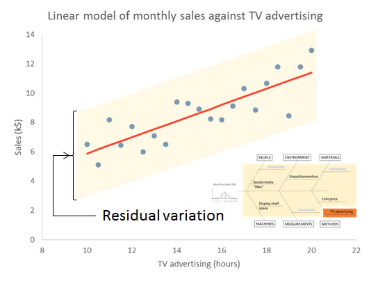
Source of Variation (2) – Residual variation
We start with the Source of Uncertainty arising from the residual variation. This is the uncertainty because of all the things we don’t know. We talked about this a lot in Part 2. We are content, for the moment, that they are sufficiently stable to form a basis for prediction. We call this common cause variation. This variation has variance s2, where s is the residual standard deviation that will be output by your regression software.
Source of Variation (3A) – Sampling error in mean
To understand the next Source of Variation we need to know a little bit about how the regression is calculated. The calculations start off with the respective means of the X values ( X̄ ) and of the Y values ( Ȳ ). Uncertainty in estimating the mean of the Y , is the next contribution to the global prediction uncertainty.
An important part of calculating the regression line is to calculate the mean of the Ys. That mean is subject to sampling error. The variance of the sampling error is the familiar result from the statistics service course.

— where n is the number of pairs of X and Y. Obviously, as we collect more and more data this term gets more and more negligible.

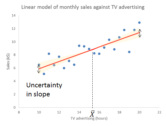
Source of Variation (3B) – Sampling error in slope
This is a bit more complicated. Skip forwards if you are already confused. Let me first give you the equation for the variance of predictions referable to sampling error in the slope.
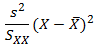
This has now introduced the mysterious sum of squares, SXX. However, before we learn exactly what this is, we immediately notice two things.
- As we move away from the centre of the training data the variance gets larger.3
- As SXX gets larger the variance gets smaller.
The reason for the increasing sampling error as we move from the mean of X is obvious from thinking about how variation in slope works. The regression line pivots on the mean. Travelling further from the mean amplifies any disturbance in the slope.
Let’s look at where SXX comes from. The sum of squares is calculated from the Xs alone without considering the Ys. It is a characteristic of the sampling frame that we used to train the model. We take the difference of each X value from the mean of X, and then square that distance. To get the sum of squares we then add up all those individual squares. Note that this is a sum of the individual squares, not their average.

Two things then become obvious (if you think about it).
- As we get more and more data, SXX gets larger.
- As the individual Xs spread out over a greater range of X, SXX gets larger.
What that (3B) term does emphasise is that even sampling error escalates as we exploit the edge of the original training data. As we extrapolate clear of the original sampling frame, the pure sampling error can quickly exceed even the residual variation.
Yet it is only a lower bound on the uncertainty in extrapolation. As we move away from the original range of Xs then, however happy we were previously with Source of Uncertainty (1), that the data was from “an environment that is sufficiently regular to be predictable”, then the question barges back in. We are now remote from our experience base in time and boundary. Nothing outside the original X-range will ever be a candidate for a comfort zone.
The fundamental theorem of prediction
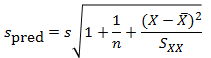
Variances, generally, add up so we can sum the three Sources of Variation (2), (3A) and (3B). That gives the variance of an individual prediction, spred2. By an individual prediction I mean that somebody gives me an X and I use the regression formula to give them the (as yet unknown) corresponding Ypred.

It is immediately obvious that s2 is common to all three terms. However, the second and third terms, the sampling errors, can be made as small as we like by collecting more and more data. Collecting more and more data will have no impact on the first term. That arises from the residual variation. The stuff we don’t yet understand. It has variance s2, where s is the residual standard deviation that will be output by your regression software.
This, I say, is the fundamental theorem of prediction. The unexplained variation provides a hard limit on the precision of forecasts.
It is then a very simple step to convert the variance into a standard deviation, spred. This is the standard error of the prediction.4,5
Now, in general, where we have a measurement or prediction z that has an uncertainty that can be characterised by a standard error u, there is an old trick for putting an interval round it. Remember that u is a measure of the variation in z. We can therefore put an interval around z as a number of standard errors, z±ku. Here, k is a constant of your choice. A prediction interval for the regression that generates prediction Ypred then becomes:
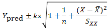
Choosing k=3 is very popular, conservative and robust.6,7 Other choices of k are available on the advice of a specialist mathematician.
It was Shewhart himself who took this all a bit further and defined tolerance intervals which contain a given proportion of future observations with a given probability.8 They are very much for the specialist.
Source of Variation (1) – Special causes
But all that assumes that we are sampling from “an environment that is sufficiently regular to be predictable”, that the residual variation is solely common cause. We checked that out on our original training data but the price of predictability is eternal vigilance. It can never be taken for granted. At any time fresh causes of variation may infiltrate the environment, or become newly salient because of some sensitising event or exotic interaction.
The real trouble with this world of ours is not that it is an unreasonable world, nor even that it is a reasonable one. The commonest kind of trouble is that it is nearly reasonable, but not quite. Life is not an illogicality; yet it is a trap for logicians. It looks just a little more mathematical and regular than it is; its exactitude is obvious, but its inexactitude is hidden; its wildness lies in wait.
G K Chesterton
The remedy for this risk is to continue plotting the residuals, the differences between the observed value and, now, the prediction. This is mandatory.
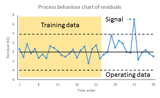
Whenever we observe a signal of a potential special cause it puts us on notice to protect the forecast-user because our ability to predict the future has been exposed as deficient and fallible. But it also presents an opportunity. With timely investigation, a signal of a possible special cause may provide deeper insight into the variation of the cause-system. That in itself may lead to identifying further factors to build into the regression and a consequential reduction in s2.
It is reducing s2, by progressively accumulating understanding of the cause-system and developing the model, that leads to more precise, and more reliable, predictions.
Notes
- Kahneman, D (2011) Thinking, Fast and Slow, Allen Lane, p240
- Hahn, G J & Meeker, W Q (1991) Statistical Intervals: A Guide for Practitioners, Wiley, p31
- In fact s2/SXX is the sampling variance of the slope. The standard error of the slope is, notoriously, s/√SXX. A useful result sometimes. It is then obvious from the figure how variation is slope is amplified as we travel father from the centre of the Xs.
- Draper, N R & Smith, H (1998) Applied Regression Analysis, 3rd ed., Wiley, pp81-83
- Hahn & Meeker (1991) p232
- Wheeler, D J (2000) Normality and the Process Behaviour Chart, SPC Press, Chapter 6
- Vysochanskij, D F & Petunin, Y I (1980) “Justification of the 3σ rule for unimodal distributions”, Theory of Probability and Mathematical Statistics 21: 25–36
- Hahn & Meeker (1991) p231

 Recently, the press reported that UK construction company Bovis Homes Group PLC have run into trouble for encouraging new homeowners to move into unfinished homes and have therefore faced a barrage of complaints about construction defects. It turns out that these practices were motivated by a desire to hit ambitious growth targets. Yet it has all had a substantial impact on trading position and mark downs for Bovis shares.1
 … is a question I often get asked. I blog here about statistics, data, quality, data quality, productivity, management and leadership. And evidence. I do it from my perspective as a practising lawyer and some people find that odd. Yet it turns out that the collaboration between law and quantitative management science is a venerable one.
 Between 1958 and 1960, 67 of the 120 inhabitants of the Chinese village of Xiaogang starved to death. But
  I had an intriguing insight into the nature of imagination the other evening when I was watching
