This blog appeared on the Royal Statistical Society website Statslife on 25 August 2015

This recent item in the New York Times has catalysed discussion among managers. The article tells of Amazon’s founder, Jeff Bezos, and his pursuit of rigorous data driven management. It also tells employees’ own negative stories of how that felt emotionally.

The New York Times says that Amazon is pervaded with abundant data streams that are used to judge individual human performance and which drive reward and advancement. They inform termination decisions too.

The recollections of former employees are not the best source of evidence about how a company conducts its business. Amazon’s share of the retail market is impressive and they must be doing something right. What everybody else wants to know is, what is it? Amazon are very coy about how they operate and there is a danger that the business world at large takes the wrong messages.

Targets

Targets are essential to business. The marketing director predicts that his new advertising campaign will create demand for 12,000 units next year. The operations director looks at her historical production data. She concludes that the process lacks the capability reliably to produce those volumes. She estimates the budget required to upgrade the process and to achieve 12,000 units annually. The executive board considers the business case and signs off the investment. Both marketing and operations directors now have a target.

Targets communicate improvement priorities. They build confidence between interfacing processes. They provide constraints and parameters that prevent the system causing harm. Harm to others or harm to itself. They allow the pace and substance of multiple business processes, and diverse entities, to be matched and aligned.

But everyone who has worked in business sees it as less simple than that. The marketing and operations directors are people.

Signal and noise

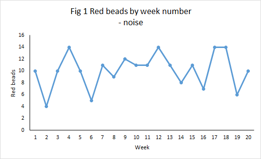
Drawing conclusions from data might be an uncontroversial matter were it not for the most common feature of data, fluctuation. Call it variation if you prefer. Business measures do not stand still. Every month, week, day and hour is different. All data features noise. Sometimes is goes up, sometimes down. A whole ecology of occult causes, weakly characterised, unknown and as yet unsuspected, interact to cause irregular variation. They are what cause a coin variously to fall “heads” or “tails”. That variation may often be stable enough, or if you like “exchangeable“, so as to allow statistical predictions to be made, as in the case of the coin toss.

If all data features noise then some data features signals. A signal is a sign, an indicator that some palpable cause has made the data stand out from the background noise. It is that assignable cause which enables inferences to be drawn about what interventions in the business process have had a tangible effect and what future innovations might cement any gains or lead to bigger prospective wins. Signal and noise lead to wholly different business strategies.

The relevance for business is that people, where not exposed to rigorous decision support, are really bad at telling the difference between signal and noise. Nobel laureate economist and psychologist Daniel Kahneman has amassed a lifetime of experimental and anecdotal data capturing noise misinterpreted as signal and judgments in the face of compelling data, distorted by emotional and contextual distractions.

Signal and accountability

It is a familiar trope of business, and government, that extravagant promises are made, impressive business cases set out and targets signed off. Yet the ultimate scrutiny as to whether that envisaged performance was realised often lacks rigour. Noise, with its irregular ups and downs, allows those seeking solace from failure to pick out select data points and cast self-serving narratives on the evidence.

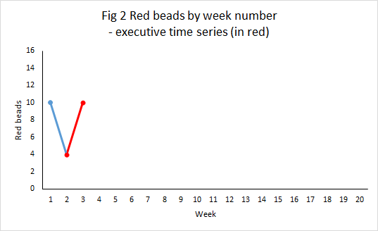
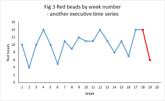
Our hypothetical marketing director may fail to achieve his target but recount how there were two individual months where sales exceeded 1,000, construct elaborate rationales as to why only they are representative of his efforts and point to purported external factors that frustrated the remaining ten reports. Pairs of individual data points can always be selected to support any story, Don Wheeler’s classic executive time series.

This is where the ability to distinguish signal and noise is critical. To establish whether targets have been achieved requires crisp definition of business measures, not only outcomes but also the leading indicators that provide context and advise judgment as to prediction reliability. Distinguishing signal and noise requires transparent reporting that allows diverse streams of data criticism. It requires a rigorous approach to characterising noise and a systematic approach not only to identifying signals but to reacting to them in an agile and sustainable manner.

Data is essential to celebrating a target successfully achieved and to responding constructively to a failure. But where noise is gifted the status of signal to confirm a fanciful business case, or to protect a heavily invested reputation, then the business is misled, costs increased, profits foregone and investors cheated.

Where employees believe that success and reward is being fudged, whether because of wishful thinking or lack of data skills, or mistakenly through lack of transparency, then cynicism and demotivation will breed virulently. Employees watch the behaviours of their seniors carefully as models of what will lead to their own advancement. Where it is deceit or innumeracy that succeed, that is what will thrive.

Noise and blame

Here is some data of the number of defects caused by production workers last month.

What is to be done about Gabriela? Move to an easier job? Perhaps retraining? Or should she be let go? And Simone? Promote to supervisor?

Well, the numbers were just random numbers that I generated. I didn’t add anything in to make Gabriela’s score higher and there was nothing in the way that I generated the data to suggest who would come top or bottom. The data are simply noise. They are the sort of thing that you might observe in a manufacturing plant that presented a “stable system of trouble”. Nothing in the data signals any behaviour, attitude, skill or diligence that Gabriela lacked or wrongly exercised. The next month’s data would likely show a different candidate for dismissal.

Mistaking signal for noise is, like mistaking noise for signal, the path to business under performance and employee disillusionment. It has a particularly corrosive effect where used, as it might be in Gabriela’s case, to justify termination. The remaining staff will be bemused as to what Gabriela was actually doing wrong and start to attach myriad and irrational doubts to all sorts of things in the business. There may be a resort to magical thinking. The survivors will be less open and less willing to share problems with their supervisors. The business itself has the costs of recruitment to replace Gabriela. The saddest aspect of the whole business is the likelihood that Gabriela’s replacement will perform better than did Gabriela, vindicating the dismissal in the mind of her supervisor. This is the familiar statistical artefact of regression to the mean. An extreme event is likely to be followed by one less extreme. Again, Kahneman has collected sundry examples of managers so deceived by singular human performance and disappointed by its modest follow-up.

It was W Edwards Deming who observed that every time you recruit a new employee you take a random sample from the pool of job seekers. That’s why you get the regression to the mean. It must be true at Amazon too as their human resources executive Mr Tony Galbato explains their termination statistics by admitting that “We don’t always get it right.” Of course, everybody thinks that their recruitment procedures are better than average. That’s a management claim that could well do with rigorous testing by data.

Further, mistaking noise for signal brings the additional business expense of over adjustment, spending money to add costly variation while degrading customer satisfaction. Nobody in the business feels good about that.

Target quality, data quality

I admitted above that the evidence we have about Amazon’s operations is not of the highest quality. I’m not in a position to judge what goes on at Amazon. But all should fix in their minds that setting targets demands rigorous risk assessment, analysis of perverse incentives and intense customer focus.

It is a sad reality that, if you set incentives perversely enough,some individuals will find ways of misreporting data. BNFL’s embarrassment with Kansai Electric and Steven Eaton’s criminal conviction were not isolated incidents.

One thing that especially bothered me about the Amazon report was the soi-disant Anytime Feedback Tool that allowed unsolicited anonymous peer appraisal. Apparently, this formed part of the “data” that determined individual advancement or termination. The description was unchallenged by Amazon’s spokesman (sic) Mr Craig Berman. I’m afraid, and I say this as a practising lawyer, unsourced and unchallenged “evidence” carries the spoor of the Star Chamber and the party purge. I would have thought that a pretty reliable method for generating unreliable data would be to maximise the personal incentives for distortion while protecting it from scrutiny or governance.

Kahneman observed that:

… we pay more attention to the content of messages than to information about their reliability, and as a result end up with a view of the world around us that is simpler and more coherent than the data justify.

It is the perverse confluence of fluctuations and individual psychology that makes statistical science essential, data analytics interesting and business, law and government difficult.