Soccer management – signal, noise and contract negotiation

Some poor data journalism here from the BBC on 28 May 2015, concerning turnover in professional soccer managers in England. “Managerial sackings reach highest level for 13 years” says the headline. A classic executive time series. What is the significance of the 13 years? Other than it being the last year with more sackings than the present.

The data was purportedly from the League Managers’ Association (LMA) and their Richard Bevan thought the matter “very concerning”. The BBC provided a chart (fair use claimed).

MgrSackingsto201503

Now, I had a couple of thoughts as soon as I saw this. Firstly, why chart only back to 2005/6? More importantly, this looked to me like a stable system of trouble (for football managers) with the possible exception of this (2014/15) season’s Championship coach turnover. Personally, I detest multiple time series on a common chart unless there is a good reason for doing so. I do not think it the best way of showing variation and/ or association.

Signal and noise

The first task of any analyst looking at data is to seek to separate signal from noise. Nate Silver made this point powerfully in his book The Signal and the Noise: The Art and Science of Prediction. As Don Wheeler put it: all data has noise; some data has signal.

Noise is typically the irregular aggregate of many causes. It is predictable in the same way as a roulette wheel. A signal is a sign of some underlying factor that has had so large an effect that it stands out from the noise. Signals can herald a fundamental unpredictability of future behaviour.

If we find a signal we look for a special cause. If we start assigning special causes to observations that are simply noise then, at best, we spend money and effort to no effect and, at worst, we aggravate the situation.

The Championship data

In any event, I wanted to look at the data for myself. I was most interested in the Championship data as that was where the BBC and LMA had been quick to find a signal. I looked on the LMA’s website and this is the latest data I found. The data only records dismissals up to 31 March of the 2014/15 season. There were 16. The data in the report gives the total number of dismissals for each preceding season back to 2005/6. The report separates out “dismissals” from “resignations” but does not say exactly how the classification was made. It can be ambiguous. A manager may well resign because he feels his club have themselves repudiated his contract, a situation known in England as constructive dismissal.

The BBC’s analysis included dismissals right up to the end of each season including 2014/15. Reading from the chart they had 20. The BBC have added some data for 2014/15 that isn’t in the LMA report and not given the source. I regard that as poor data journalism.

I found one source of further data at website The Sack Race. That told me that since the end of March there had been four terminations.

Manager Club Termination Date
Malky Mackay Wigan Athletic Sacked 6 April
Lee Clark Blackpool Resigned 9 May
Neil Redfearn Leeds United Contract expired 20 May
Steve McClaren Derby County Sacked 25 May

As far as I can tell, “dismissals” include contract non-renewals and terminations by mutual consent. There are then a further three dismissals, not four. However, Clark left Blackpool amid some corporate chaos. That is certainly a termination that is classifiable either way. In any event, I have taken the BBC figure at face value though I am alerted as to some possible data quality issues here.
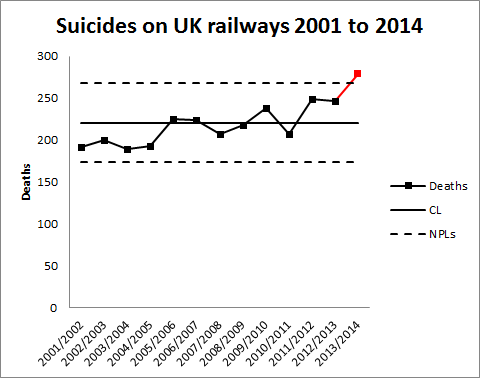
Signal and noise

Looking at the Championship data, this was the process behaviour chart, plotted as an individuals chart.

MgrSackingsto201503

There is a clear signal for the 2014/15 season with an observation, 20 dismissals,, above the upper natural process limit of 19.18 dismissals. Where there is a signal we should seek a special cause. There is no guarantee that we will find a special cause. Data limitations and bounded rationality are always constraints. In fact, there is no guarantee that there was a special cause. The signal could be a false positive. Such effects cannot be eliminated. However, signals efficiently direct our limited energy for, what Daniel Kahneman calls, System 2 thinking towards the most promising enquiries.

Analysis

The BBC reports one narrative woven round the data.

Bevan said the current tenure of those employed in the second tier was about eight months. And the demand to reach the top flight, where a new record £5.14bn TV deal is set to begin in 2016, had led to clubs hitting the “panic button” too quickly.

It is certainly a plausible view. I compiled a list of the dismissals and non-renewals, not the resignations, with data from Wikipedia and The Sack Race. I only identified 17 which again suggests some data quality issue around classification. I have then charted a scatter plot of date of dismissal against the club’s then league position.

MgrSackings201415

It certainly looks as though risk of relegation is the major driver for dismissal. Aside from that, Watford dismissed Billy McKinlay after only two games when they were third in the league, equal on points with the top two. McKinlay had been an emergency appointment after Oscar Garcia had been compelled to resign through ill health. Watford thought they had quickly found a better manager in Slavisa Jokanovic. Watford ended the season in second place and were promoted to the Premiership.

There were two dismissals after the final game on 2 May by disappointed mid-table teams. Beyond that, the only evidence for impulsive managerial changes in pursuit of promotion is the three mid-season, mid-table dismissals.

Club league position
Manager Club On dismissal At end of season
Nigel Adkins Reading 16 19
Bob Peeters Charlton Athletic 14 12
Stuart Pearce Nottingham Forrest 12 14

A table that speaks for itself. I am not impressed by the argument that there has been the sort of increase in panic sackings that Bevan fears. Both Blackpool and Leeds experienced chaotic executive management which will have resulted in an enhanced force of mortality on their respective coaches. That along with the data quality issues and the technical matter I have described below lead me to feel that there was no great enhanced threat to the typical Championship manager in 2014/15.

Next season I would expect some regression to the mean with a lower number of dismissals. Not much of a prediction really but that’s what the data tells me. If Bevan tries to attribute that to the LMA’s activism them I fear that he will be indulging in Langian statistical analysis. Will he be able to resist?

Techie bit

I have a preference for individuals charts but I did also try plotting the data on an np-chart where I found no signal. It is trite service-course statistics that a Poisson distribution with mean λ has standard deviation √λ so an upper 3-sigma limit for a (homogeneous) Poisson process with mean 11.1 dismissals would be 21.1 dismissals. Kahneman has cogently highlighted how people tend to see patterns in data as signals even where they are typical of mere noise. In this case I am aware that the data is not atypical of a Poisson process so I am unsurprised that I failed to identify a special cause.

A Poisson process with mean 11.1 dismissals is a pretty good model going forwards and that is the basis I would press on any managers in contract negotiations.

Of course, the clubs should remember that when they look for a replacement manager they will then take a random sample from the pool of job seekers. Really!

Data and anecdote revisited – the case of the lime jellybean

JellyBellyBeans.jpgI have already blogged about the question of whether data is the plural of anecdote. Then I recently came across the following problem in the late Richard Jeffrey’s marvellous little book Subjective Probability: The Real Thing (2004, Cambridge) and it struck me as a useful template for thinking about data and anecdotes.

The problem looks like a staple of elementary statistics practice exercises.

You are drawing a jellybean from a bag in which you know half the beans are green, all the lime flavoured ones are green and the green ones are equally divided between lime and mint flavours.

You draw a green bean. Before you taste it, what is the probability that it is lime flavoured?

A mathematically neat answer would be 50%. But what if, asked Jeffrey, when you drew the green bean you caught a whiff of mint? Or the bean was a particular shade of green that you had come to associate with “mint”. Would your probability still be 50%?

The given proportions of beans in the bag are our data. The whiff of mint or subtle colouration is the anecdote.

What use is the anecdote?

It would certainly be open to a participant in the bean problem to maintain the 50% probability derived from the data and ignore the inferential power of the anecdote. However, the anecdote is evidence that we have and, if we choose to ignore it simply because it is difficult to deal with, then we base our assessment of risk on a more restricted picture than that actually available to us.

The difficulty with the anecdote is that it does not lead to any compelling inference in the same way as do the mathematical proportions. It is easy to see how the bean proportions would give rise to a quite extensive consensus about the probability of “lime”. There would be more variety in individual responses to the anecdote, in what weight to give the evidence and in what it tended to imply.

That illustrates the tension between data and anecdote. Data tends to consensus. If there is disagreement as to its weight and relevance then the community is likely to divide into camps rather than exhibit a spectrum of views. Anecdote does not lead to such a consensus. Individuals interpret anecdotes in diverse ways and invest them with varying degrees of credence.

Yet, the person who is best at weighing and interpreting the anecdotal evidence has the advantage over the broad community who are in agreement about what the proportion data tells them. It will often be the discipline specialist who is in the best position to interpret an anecdote.

From anecdote to data

One of the things that the “mint” anecdote might do is encourage us to start collecting future data on what we smelled when a bean was drawn. A sequence of such observations, along with the actual “lime/ mint” outcome, potentially provides a potent decision support mechanism for future draws. At this point the anecdote has been developed into data.

This may be a difficult process. The whiff of mint or subtle colouration could be difficult to articulate but recognising its significance (sic) is the beginning of operationalising and sharing.

Statistician John Tukey advocated the practice of exploratory data analysis (EDA) to identify such anecdotal evidence before settling on a premature model. As he observed:

The greatest value of a picture is when it forces us to notice what we never expected to see.

Of course, the person who was able to use the single anecdote on its own has the advantage over those who had to wait until they had compelling data. Data that they share with everybody else who has the same idea.

Data or anecdote

When I previously blogged about this I had trouble in coming to any definition that distinguished data and anecdote. Having reflected, I have a modest proposal. Data is the output of some reasonably well-defined process. Anecdote isn’t. It’s not clear how it was generated.

We are not told by what process the proportion of beans was established but I am willing to wager that it was some form of counting.

If we know the process generating evidence then we can examine its biases, non-responses, precision, stability, repeatability and reproducibility. Anecdote we cannot. It is because we can characterise the measurement process, through measurement systems analysis, that we can assess its reliability and make appropriate allowances and adjustments for its limitations. An assessment that most people will agree with most of the time. Because the most potent tools for assessing the reliability of evidence are absent in the case of anecdote, there are inherent difficulties in its interpretation and there will be a spectrum of attitudes from the community.

However, having had our interest pricked by the anecdote, we can set up a process to generate data.

Borrowing strength again

Using an anecdote as the basis for further data generation is one approach to turning anecdote into reliable knowledge. There is another way.

Today in the UK, a jury of 12 found nurse Victorino Chua, beyond reasonable doubt, guilty of poisoning 21 of his patients with insulin. Two died. There was no single compelling piece of evidence put before the jury. It was all largely circumstantial. The prosecution had sought to persuade the jury that those various items of circumstantial evidence reinforced each other and led to a compelling inference.

This is a common situation in litigation where there is no single conclusive piece of data but various pieces of circumstantial evidence that have to be put together. Where these reinforce, they inherit borrowing strength from each other.

Anecdotal evidence is not really the sort of evidence we want to have. But those who know how to use it are way ahead of those embarrassed by it.

Data is the plural of anecdote, either through repetition or through borrowing.

Royal babies and the wisdom of crowds

Prince George of Cambridge with wombat plush toy (crop).jpgIn 2004 James Surowiecki published a book with the unequivocal title The Wisdom of Crowds: Why the Many Are Smarter Than the Few and How Collective Wisdom Shapes Business, Economies, Societies and Nations. It was intended as a gloss on Charles Mackay’s 1841 book Extraordinary Popular Delusions and the Madness of Crowds. Both books are essential reading for any risk professional.

I am something of a believer in the wisdom of crowds. The other week I was fretting about the possible relegation of English Premier League soccer club West Bromwich Albion. It’s an emotional and atavistic tie for me. I always feel there is merit, as part of my overall assessment of risk, in checking online bookmakers’ odds. They surely represent the aggregated risk assessment of gamblers if nobody else. I was relieved that bookmakers were offering typically 100/1 against West Brom being relegated. My own assessment of risk is, of course, contaminated with personal anxiety so I was pleased that the crowd was more phlegmatic.

However, while I was on the online bookmaker’s website, I couldn’t help but notice that they were also accepting bets on the imminent birth of the royal baby, the next child of the Duke and Duchess of Cambridge. It struck me as weird that anyone would bet on the sex of the royal baby. Surely this was a mere coin toss, though I know that people will bet on that. Being hopelessly inquisitive I had a look. I was somewhat astonished to find these odds being offered (this was 22 April 2015, ten days before the royal birth).

odds implied probability
Girl 1/2 0.67
Boy 6/4 0.40
 Total 1.07

Here I have used the usual formula for converting between odds and implied probabilities: odds of m / n against an event imply a probability of n / (m + n) of the event occurring. Of course, the principle of finite additivity requires that probabilities add up to one. Here they don’t and there is an overround of 7%. Like the rest of us, bookmakers have to make a living and I was unsurprised to find a Dutch book.

The odds certainly suggested that the crowd thought a girl manifestly more probable than a boy. Bookmakers shorten the odds on the outcome that is attracting the money to avoid a heavy payout on an event that the crowd seems to know something about.

Historical data on sex ratio

I started, at this stage, to doubt my assumption that boy/ girl represented no more than a coin toss, 50:50, an evens bet. As with most things, sex ratio turns out to be an interesting subject. I found this interesting research paper which showed that sex ratio was definitely dependent on factors such as the age and ethnicity of the mother. The narrative of this chart was very interesting.

Sex ratio

However, the paper confirmed that the sex of a baby is independent of previous births, conditioned on the factors identified, and that the ratio of girls to boys is nowhere and no time greater than 1,100 to 1000, about 52% girls.

So why the odds?

Bookmakers lengthen the odds on the outcome attracting the smaller value of bets in order to encourage stakes on the less fancied outcomes, on which there is presumably less risk of having to pay out. At odds of 6/4, a punter betting £10 on a boy would receive his stake back plus £15 ( = 6 × £10 / 4 ). If we assume an equal chance of boy or girl then that is an expected return of £12.50 ( = 0.5 × £25 ) for a £10.00 stake. I’m not sure I’d seen such a good value wager since we all used to bet against Tim Henman winning Wimbledon.

Ex ante there are two superficially suggestive explanations as to the asymmetry in the odds. At least this is all my bounded rationality could imagine.

  • A lot of people (mistakenly) thought that the run of five male royal births (Princes Andrew, Edward, William, Harry and George) escalated the probability of a girl being next. “It was overdue.”
  • A lot of people believed that somebody “knew something” and that they knew what it was.

In his book about cognitive biases in decision making (Thinking, Fast and Slow, Allen Lane, 2011) Nobel laureate economist Daniel Kahneman describes widespread misconceptions concerning randomness of boy/ girl birth outcomes (at p115). People tend to see regularity in sequences of data as evidence of non-randomness, even where patterns are typical of, and unsurprising in, random events.

I had thought that there could not be sufficient gamblers who would be fooled by the baseless belief that a long run of boys made the next birth more likely to be a girl. But then Danny Finkelstein reminded me (The (London) Times, Saturday 25 April 2015) of a survey of UK politicians that revealed their limited ability to deal with chance and probabilities. Are politicians more or less competent with probabilities than online gamblers? That is a question for another day. I could add that the survey compared politicians of various parties but we have an on-going election campaign in the UK at the moment so I would, in the interest of balance, invite my voting-age UK readers not to draw any inferences therefrom.

The alternative is the possibility that somebody thought that somebody knew something. The parents avowed that they didn’t know. Medical staff may or may not have. The sort of people who work in VIP medicine in the UK are not the sort of people who divulge information. But one can imagine that a random shift in sentiment, perhaps because of the misconception that a girl was “overdue”, and a consequent drift in the odds, could lead others to infer that there was insight out there. It is not completely impossible. How many other situations in life and business does that model?

It’s a girl!

The wisdom of crowds or pure luck? We shall never know. I think it was Thomas Mann who observed that the best proof of the genuineness of a prophesy was that it turned out to be false. Had the royal baby been a boy we could have been sure that the crowd was mad.

To be complete, Bayes’ theorem tells us that the outcome should enhance our degree of belief in the crowd’s wisdom. But it is a modest increase (Bayes’ factor of 2, 3 deciban after Alan Turing’s suggestion) and as we were most sceptical before we remain unpersuaded.

In his book, Surowiecki identified five factors that can impair crowd intelligence. One of these is homogeneity. Insufficient diversity frustrates the inherent virtue on which the principle is founded. I wonder how much variety there is among online punters? Similarly, where judgments are made sequentially there is a danger of influence. That was surely a factor at work here. There must also have been an element of emotion, the factor that led to all those unrealistically short odds on Henman at Wimbledon on which the wise dined so well.

But I’m trusting that none of that applies to the West Brom odds.

UK railway suicides – 2014 update

It’s taken me a while to sit down and blog about this news item from October 2014: Sharp Rise in Railway Suicides Say Network Rail . Regular readers of this blog will know that I have followed this data series closely in 2013 and 2012.

The headline was based on the latest UK government data. However, I baulk at the way these things are reported by the press. The news item states as follows.

The number of people who have committed suicide on Britain’s railways in the last year has almost reached 300, Network Rail and the Samaritans have warned. Official figures for 2013-14 show there have already been 279 suicides on the UK’s rail network – the highest number on record and up from 246 in the previous year.

I don’t think it’s helpful to characterise 279 deaths as “almost … 300”, where there is, in any event, no particular significance in the number 300. It arbitrarily conveys the impression that some pivotal threshold is threatened. Further, there is no especial significance in an increase from 246 to 279 deaths. Another executive time series. Every one of the 279 is a tragedy as is every one of the 246. The experience base has varied from year to year and there is no surprise that it has varied again. To assess the tone of the news report I have replotted the data myself.

RailwaySuicides3

Readers should note the following about the chart.

  • Some of the numbers for earlier years have been updated by the statistical authority.
  • I have recalculated natural process limits as there are still no more than 20 annual observations.
  • There is now a signal (in red) of an observation above the upper natural process limit.

The news report is justified, unlike the earlier ones. There is a signal in the chart and an objective basis for concluding that there is more than just a stable system of trouble. There is a signal and not just noise.

As my colleague Terry Weight always taught me, a signal gives us license to interpret the ups and downs on the chart. There are two possible narratives that immediately suggest themselves from the chart.

  • A sudden increase in deaths in 2013/14; or
  • A gradual increasing trend from around 200 in 2001/02.

The chart supports either story. To distinguish would require other sources of information, possibly historical data that can provide some borrowing strength, or a plan for future data collection. Once there is a signal, it makes sense to ask what was its cause. Building  a narrative around the data is a critical part of that enquiry. A manager needs to seek the cause of the signal so that he or she can take action to improve system outcomes. Reliably identifying a cause requires trenchant criticism of historical data.

My first thought here was to wonder whether the railway data simply reflected an increasing trend in suicide in general. Certainly a very quick look at the data here suggests that the broader trend of suicides has been downwards and certainly not increasing. It appears that there is some factor localised to railways at work.

I have seen proposals to repeat a strategy from Japan of bathing railway platforms with blue light. I have not scrutinised the Japanese data but the claims made in this paper and this are impressive in terms of purported incident reduction. If these modifications are implemented at British stations we can look at the chart to see whether there is a signal of fewer suicides. That is the only real evidence that counts.

Those who were advocating a narrative of increasing railway suicides in earlier years may feel vindicated. However, until this latest evidence there was no signal on the chart. There is always competition for resources and directing effort on a false assumptions leads to misallocation. Intervening in a stable system of trouble, a system featuring only noise, on the false belief that there is a signal will usually make the situation worse. Failing to listen to the voice of the process on the chart risks diverting vital resources and using them to make outcomes worse.

Of course, data in terms of time between incidents is much more powerful in spotting an early signal. I have not had the opportunity to look at such data but it would have provided more, better and earlier evidence.

Where there is a perception of a trend there will always be an instinctive temptation to fit a straight line through the data. I always ask myself why this should help in identifying the causes of the signal. In terms of analysis at this stage I cannot see how it would help. However, when we come to look for a signal of improvement in future years it may well be a helpful step.

Proposition 65

WarningPoster1I had break from posting following my recent family vacation to California. While I was out there I noticed this rather alarming notice at a beach hotel and restaurant in Santa Monica. After a bit of research it turned out that the notice was motivated by California Proposition 65 (1986). Everywhere we went in California we saw similar notices.

I stand in this issue not solely as somebody professionally involved in risk but also as an individual concerned for his own health and that of his family. If there is an audience for warnings of harm then it is me.

I am aware of having embarked on a huge topic here but, as I say, it is as a concerned consumer of risk advice. The notice, and I hesitate to call it a warning, was unambiguous. Apparently, this hotel, teeming with diners and residents enjoying the pacific coast, did contain chemicals emphatically “known” to cause cancer, birth defects or reproductive harm. Yet for such dreadful risks to be present the notice gave alarmingly vague information. I saw that a brochure was available within the hotel but my wife was unwilling to indulge my professional interest. I suspect that most visitors showed even less curiosity.

As far as discharging any legal duty goes, vague notices offer no protection to anybody. In the English case of Vacwell Engineering Co. Ltd v B.D.H. Chemicals Ltd [1969] 3 All ER 1681, Vacwell purchased ampules of boron tribromide from B.D.H.. The ampules bore the label “Harmful Vapour”. While the ampules were being washed, one was dropped into a sink where it fractured allowing the contents to come into contact with water. Mixing water with boron tribromide caused an explosion that killed one employee and extensively damaged a laboratory building. The label had given B.D.H. no information as to the character or possible severity of the hazard, nor any specific details that would assist in avoiding the consequences.

Likewise the Proposition 65 notice gives me no information on the severity of the hazard. There is a big difference between “causing” cancer and posing a risk of cancer. The notice doesn’t tell me whether cancer is an inevitable consequence of exposure or whether I should just shorten my odds against mortality. There is no quantification of risk on which I can base my own decisions.

Nor does the notice give me any guidance on what to do to avoid or mitigate the risk. Will stepping foot inside the premises imperil my health? Or are there only certain areas that are hazardous? Are these delineated with further and more specific warnings? Or even ultimately segregated in secure areas? Am I even safe immediately outside the premises? Ten yards away? A mile? I have to step inside to acquire the brochure so I think I should be told.

The notice ultimately fulfils no socially useful purpose whatever. I looked at the State of California’s own website on the matter but found it too opaque to extract any useful information within the time I was willing to spend on it, which I suspect is more time than most of the visitors who find their way there.

It is most difficult for members of the public, even those engaged and interested, to satisfy themselves as to the science on these matters. The risks fall within what John Adams at University College London characterises as risks that are known to science but on which normal day to day intuition is of little use. The difficulty we all have is that our reflection on the risks is conditioned on the anecdotal hearsay that we pick up along the way. I have looked before at the question of whether anecdote is data.

In 1962, Rachel Carson published the book Silent Spring. The book aggregated anecdotes and suggestive studies leading Carson to infer that industrial pesticides were harming agriculture, wildlife and human health. Again, proper evaluation of the case she advanced demands more attention to scientific detail than any lay person is willing to spare. However, the fear she articulated lingers and conditions our evaluation of other claims. It seems so plausible that synthetic chemicals developed for lethal effect, rather than evolved in symbiosis with the natural world, would pose a threat to human life and be an explanation for increasing societal morbidity.

However, where data is sparse and uncertain, it is important to look for other sources of information that we can “borrow” to add “strength” to our preliminary assessment (Persi Diaconis’ classic paper Theories of Data Analysis: From Magical Thinking through Classical Statistics has some lucid insights on this). I found the Cancer Research UK website provided me with some helpful borrowing strength. Cancer is becoming more prevalent largely because we are living longer. Cancer Research helpfully referred me to this academic research published in the British Journal of Cancer.

Despite the difficulty in disentangling and interpreting data on specific risks of alleged pathogens we have the strength of borrowing from life expectancy data. Life expectancy has manifestly improved in the half century since Carson’s book, belying her fear of a toxic catastrophe flowing from our industrialised society. I think that is why there was so much indifference to the Santa Monica notice.

I should add that, inside the hotel, I spotted five significant trip hazards. I suspect these posed a much more substantial threat to visitors’ wellbeing than the virtual risks of contamination with hotel carcinogens.