Regression done right: Part 2: Is it worth the trouble?

In Part 1 I looked at linear regression from the point of view of machine learning and asked the question whether the data was from “An environment that is sufficiently regular to be predictable.”1 The next big question is whether it was worth it in the first place.

Variation explained

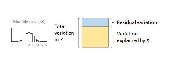
We previously looked at regression in terms of explaining variation. The original Big Y was beset with variation and uncertainty. We believed that some of that variation could be “explained” by a Big X. The linear regression split the variation in Y into variation that was explained by X and residual variation whose causes are as yet obscure.

I slipped in the word “explained”. Here it really means that we can draw a straight line relationship between X and Y. Of course, it is trite analytics that “association is not causation”. As long ago as 1710, Bishop George Berkeley observed that:2

The Connexion of Ideas does not imply the Relation of Cause and Effect, but only a Mark or Sign of the Thing signified.

Causation turns out to be a rather slippery concept, as all lawyers know, so I am going to leave it alone for the moment. There is a rather good discussion by Stephen Stigler in his recent book The Seven Pillars of Statistical Wisdom.3

That said, in real world practical terms there is not much point bothering with this if the variation explained by the X is small compared to the original variation in the Y with the majority of the variation still unexplained in the residuals.

Measuring variation

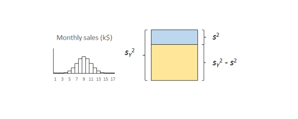
A useful measure of the variation in a quantity is its variance, familiar from the statistics service course. Variance is a good straightforward measure of the financial damage that variation does to a business.4 It also has the very nice property that we can add variances from sundry sources that aggregate together. Financial damage adds up. The very useful job that linear regression does is to split the variance of Y, the damage to the business that we captured with the histogram, into two components:

  • The contribution from X; and
  • The contribution of the residuals.

RegressionBlock1
The important thing to remember is that the residual variation is not some sort of technical statistical artifact. It is the aggregate of real world effects that remain unexamined and which will continue to cause loss and damage.
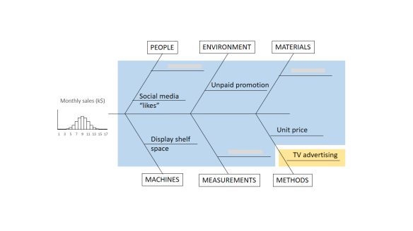
RegressionIshikawa2

Techie bit

Variance is the square of standard deviation. Your linear regression software will output the residual standard deviation, s, sometimes unhelpfully referred to as the residual standard error. The calculations are routine.5 Square s to get the residual variance, s2. The smaller is s2, the better. A small s2 means that not much variation remains unexplained. Small s2 means a very good understanding of the cause system. Large s2 means that much variation remains unexplained and our understanding is weak.
RegressionBlock2

The coefficient of determination

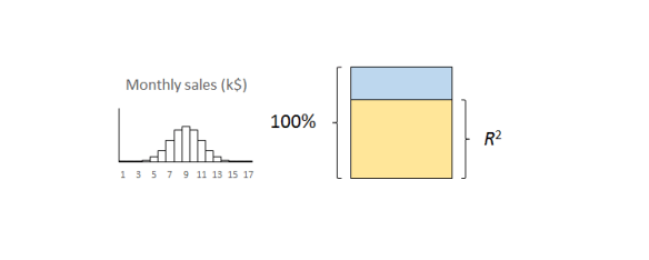
So how do we decide whether s2 is “small”? Dividing the variation explained by X by the total variance of Y, sY2,  yields the coefficient of determination, written as R2.6 That is a bit of a mouthful so we usually just call it “R-squared”. R2 sets the variance in Y to 100% and expresses the explained variation as a percentage. Put another way, it is the percentage of variation in Y explained by X.
RegressionBlock3The important thing to remember is that the residual variation is not a statistical artifact of the analysis. It is part of the real world business system, the cause-system of the Ys.7 It is the part on which you still have little quantitative grasp and which continues to hurt you. Returning to the cause and effect diagram, we picked one factor X to investigate and took its influence out of the data. The residual variation is the variation arising from the aggregate of all the other causes.

As we shall see in more detail in Part 3, the residual variation imposes a fundamental bound on the precision of predictions from the model. It turns out that s is the limiting standard error of future predictions

Whether your regression was a worthwhile one or not so you will want to probe the residual variation further. A technique like DMAIC works well. Other improvement processes are available.

So how big should R2 be? Well that is a question for your business leaders not a statistician. How much does the business gain financially from being able to explain just so much variation in the outcome? Anybody with an MBA should be able to answer this so you should have somebody in your organisation who can help.

The correlation coefficient

Some people like to take the square root of R2 to obtain what they call a correlation coefficient. I have never been clear as to what this was trying to achieve. It always ends up telling me less than the scatter plot. So why bother? R2 tells me something important that I understand and need to know. Leave it alone.

What about statistical significance?

I fear that “significance” is, pace George Miller, “a word worn smooth by many tongues”. It is a word that I try to avoid. Yet it seems a natural practice for some people to calculate a p-value and ask whether the regression is significant.

I have criticised p-values elsewhere. I might calculate them sometimes but only because I know what I am doing. The terrible fact is that if you collect sufficient data then your regression will eventually be significant. Statistical significance only tells me that you collected a lot of data. That’s why so many studies published in the press are misleading. Collect enough data and you will get a “significant” result. It doesn’t mean it matters in the real world.

R2 is the real world measure of sensible trouble (relatively) impervious to statistical manipulation. I can make p as small as I like just by collecting more and more data. In fact there is an equation that, for any given R2, links p and the number of observations, n, for linear regression.8

FvR2 equation

Here, Fμ, ν(x) is the F-distribution with μ and ν degrees of freedom. A little playing about with that equation in Excel will reveal that you can make p as small as you like without R2 changing at all. Simply by making n larger. Collecting data until p is small is mere p-hacking. All p-values should be avoided by the novice. R2 is the real world measure (relatively) impervious to statistical manipulation. That is what I am interested in. And what your boss should be interested in.

Next time

Once we are confident that our regression model is stable and predictable, and that the regression is worth having, we can move on to the next stage.

Next time I shall look at prediction intervals and how to assess uncertainty in forecasts.

References

  1. Kahneman, D (2011) Thinking, Fast and Slow, Allen Lane, p240
  2. Berkeley, G (1710) A Treatise Concerning the Principles of Human Knowledge, Part 1, Dublin
  3. Stigler, S M (2016) The Seven Pillars of Statistical Wisdom, Harvard University Press, pp141-148
  4. Taguchi, G (1987) The System of Experimental Design: Engineering Methods to Optimize Quality and Minimize Costs, Quality Resources
  5. Draper, N R & Smith, H (1998) Applied Regression Analysis, 3rd ed., Wiley, p30
  6. Draper & Smith (1998) p33
  7. For an appealing discussion of cause-systems from a broader cultural standpoint see: Bostridge, I (2015) Schubert’s Winter Journey: Anatomy of an Obsession, Faber, pp358-365
  8. Draper & Smith (1998) p243

Regression done right: Part 1: Can I predict the future?

I recently saw an article in the Harvard Business Review called “Refresher on Regression Analysis”. I thought it was horrible so I wanted to set the record straight.

Linear regression from the viewpoint of machine learning

Linear regression is important, not only because it is a useful tool in itself, but because it is (almost) the simplest statistical model. The issues that arise in a relatively straightforward form are issues that beset the whole of statistical modelling and predictive analytics. Anyone who understands linear regression properly is able to ask probing questions about more complicated models. The complex internal algorithms of Kalman filters, ARIMA processes and artificial neural networks are accessible only to the specialist mathematician. However, each has several general features in common with simple linear regression. A thorough understanding of linear regression enables a due diligence of the claims made by the machine learning advocate. Linear regression is the paradigmatic exemplar of machine learning.

There are two principal questions that I want to talk about that are the big takeaways of linear regression. They are always the first two questions to ask in looking at any statistical modelling or machine learning scenario.

  1. What predictions can I make (if any)?
  2. Is it worth the trouble?

I am going to start looking at (1) in this blog and complete it in a future Part 2. I will then look at (2) in a further Part 3.

Variation, variation, variation

Variation is a major problem for business, the tendency of key measures to fluctuate irregularly. Variation leads to uncertainty. Will the next report be high or low? Or in the middle? Because of the uncertainty we have to allow safety margins or swallow some non-conformancies. We have good days and bad days, good products and not so good. We have to carry costly working capital because of variation in cash flow. And so on.

We learned in our high school statistics class to characterise variation in a key process measure, call it the Big Y, by an histogram of observations. Perhaps we are bothered by the fluctuating level of monthly sales.

RegressionHistogram

The variation arises from a whole ecology of competing and interacting effects and factors that we call the cause-system of the outcome. In general, it is very difficult to single out individual factors as having been the cause of a particular observation, so entangled are they. It is still useful to capture them for reference on a cause and effect diagram.

RegressionIshikawa

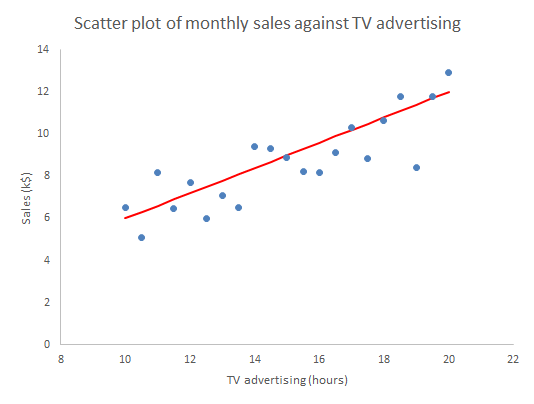
One of the strengths of the cause and effect diagram is that it may prompt the thought that one of the factors is particularly important, call it Big X, perhaps it is “hours of TV advertising” (my age is showing). Motivated by that we can generate a sample of corresponding measurements data of both the Y and X and plot them on a scatter plot.

RegressionScatter1

Well what else is there to say? The scatter plot shows us all the information in the sample. Scatter plots are an important part of what statistician John Tukey called Exploratory Data Analysis (EDA). We have some hunches and ideas, or perhaps hardly any idea at all, and we attack the problem by plotting the data in any way we can think of. So much easier now than when W Edwards Deming wrote:1

[Statistical practice] means tedious work, such as studying the data in various forms, making tables and charts and re-making them, trying to use and preserve the evidence in the results and to be clear enough to the reader: to endure disappointment and discouragement.

Or as Chicago economist Ronald Coase put it.

If you torture the data enough, nature will always confess.

The scatter plot is a fearsome instrument of data torture. It tells me everything. It might even tempt me to think that I have a basis on which to make predictions.

Prediction

In machine learning terms, we can think of the sample used for the scatter plot as a training set of data. It can be used to set up, “train”, a numerical model that we will then fix and use to predict future outcomes. The scatter plot strongly suggests that if we know a future X alone we can have a go at predicting the corresponding future Y. To see that more clearly we can draw a straight line by hand on the scatter plot, just as we did in high school before anybody suggested anything more sophisticated.

RegressionScatter2

Given any particular X we can read off the corresponding Y.

RegressionScatter3

The immediate insight that comes from drawing in the line is that not all the observations lie on the line. There is variation about the line so that there is actually a range of values of Y that seem plausible and consistent for any specified X. More on that in Parts 2 and 3.

In understanding machine learning it makes sense to start by thinking about human learning. Psychologists Gary Klein and Daniel Kahneman investigated how firefighters were able to perform so successfully in assessing a fire scene and making rapid, safety critical decisions. Lives of the public and of other firefighters were at stake. This is the sort of human learning situation that machines, or rather their expert engineers, aspire to emulate. Together, Klein and Kahneman set out to describe how the brain could build up reliable memories that would be activated in the future, even in the agony of the moment. They came to the conclusion that there are two fundamental conditions for a human to acquire a skill.2

  • An environment that is sufficiently regular to be predictable.
  • An opportunity to learn these regularities through prolonged practice

The first bullet point is pretty much the most important idea in the whole of statistics. Before we can make any prediction from the regression, we have to be confident that the data has been sampled from “an environment that is sufficiently regular to be predictable”. The regression “learns” from those regularities, where they exist. The “learning” turns out to be the rather prosaic mechanics of matrix algebra as set out in all the standard texts.3 But that, after all, is what all machine “learning” is really about.

Statisticians capture the psychologists’ “sufficiently regular” through the mathematical concept of exchangeability. If a process is exchangeable then we can assume that the distribution of events in the future will be like the past. We can project our historic histogram forward. With regression we can do better than that.

Residuals analysis

Formally, the linear regression calculations calculate the characteristics of the model:

Y = mX + c + “stuff”

The “mX+c” bit is the familiar high school mathematics equation for a straight line. The “stuff” is variation about the straight line. What the linear regression mathematics does is (objectively) to calculate the m and c and then also tell us something about the “stuff”. It splits the variation in Y into two components:

  • What can be explained by the variation in X; and
  • The, as yet unexplained, variation in the “stuff”.

The first thing to learn about regression is that it is the “stuff” that is the interesting bit. In 1849 British astronomer Sir John Herschel observed that:

Almost all the greatest discoveries in astronomy have resulted from the consideration of what we have elsewhere termed RESIDUAL PHENOMENA, of a quantitative or numerical kind, that is to say, of such portions of the numerical or quantitative results of observation as remain outstanding and unaccounted for after subducting and allowing for all that would result from the strict application of known principles.

The straight line represents what we guessed about the causes of variation in Y and which the scatter plot confirmed. The “stuff” represents the causes of variation that we failed to identify and that continue to limit our ability to predict and manage. We call the predicted Ys that correspond to the measured Xs, and lie on the fitted straight line, the fits.

fiti = mXic

The residual values, or residuals, are obtained by subtracting the fits from the respective observed Y values. The residuals represent the “stuff”. Statistical software does this for us routinely. If yours doesn’t then bin it.

residuali = Yi – fiti

RegressionScatter4

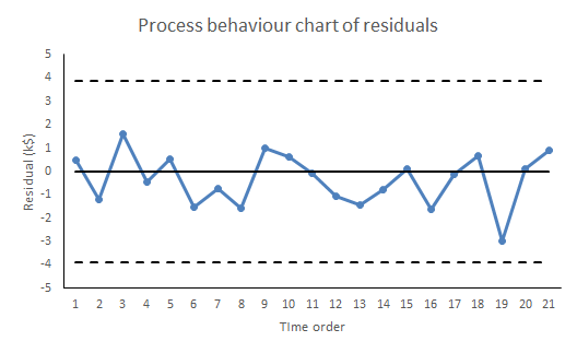
There are a number of properties that the residuals need to satisfy for the regression to work. Investigating those properties is called residuals analysis.4 As far as use for prediction in concerned, it is sufficient that the “stuff”, the variation about the straight line, be exchangeable.5 That means that the “stuff” so far must appear from the data to be exchangeable and further that we have a rational belief that such a cause system will continue unchanged into the future. Shewhart charts are the best heuristics for checking the requirement for exchangeability, certainly as far as the historical data is concerned. Our first and, be under no illusion, mandatory check on the ability of the linear regression, or any statistical model, to make predictions is to plot the residuals against time on a Shewhart chart.

RegressionPBC

If there are any signals of special causes then the model cannot be used for prediction. It just can’t. For prediction we need residuals that are all noise and no signal. However, like all signals of special causes, such will provide an opportunity to explore and understand more about the cause system. The signal that prevents us from using this regression for prediction may be the very thing that enables an investigation leading to a superior model, able to predict more exactly than we ever hoped the failed model could. And even if there is sufficient evidence of exchangeability from the training data, we still need to continue vigilance and scrutiny of all future residuals to look out for any novel signals of special causes. Special causes that arise post-training provide fresh information about the cause system while at the same time compromising the reliability of the predictions.

Thorough regression diagnostics will also be able to identify issues such as serial correlation, lack of fit, leverage and heteroscedasticity. It is essential to regression and its ommision is intolerable. Residuals analysis is one of Stephen Stigler’s Seven Pillars of Statistical Wisdom.6 As Tukey said:

The greatest value of a picture is when it forces us to notice what we never expected to see.

To come:

Part 2: Is my regression significant? … is a dumb question.
Part 3: Quantifying predictions with statistical intervals.

References

  1. Deming, W E (‎1975) “On probability as a basis for action”, The American Statistician 29(4) pp146-152
  2. Kahneman, D (2011) Thinking, Fast and Slow, Allen Lane, p240
  3. Draper, N R & Smith, H (1998) Applied Regression Analysis, 3rd ed., Wiley, p44
  4. Draper & Smith (1998) Chs 2, 8
  5. I have to admit that weaker conditions may be adequate in some cases but these are far beyond any other than a specialist mathematician.
  6. Stigler, S M (2016) The Seven Pillars of Statistical Wisdom, Harvard University Press, Chapter 7